Relational Clocks in a Quantum Ledger: Construction, Preparation and the Limits of Energy Universality
David Elliman · Neuro-Symbolic Ltd · 10 November 2026
Summary and scope
A stationary quantum state can describe change through correlations between a clock and the system it measures. This observation leaves a constructive question: can elementary exchanges with a reservoir supply the clock's energies, its correlations and its response to other records, rather than having each ingredient specified separately? We investigate finite quantum registers whose interactions are reversible transactions, without assigning them positions or a spatial geometry. A vacancy counterpart of a three-record rule produces complementary clock energies, and a matching exchange selects the correlated state above a calculable threshold. Selection does not imply preparation: closed evolution preserves the target population, and a conserved symmetry blocks preparation by the tested finite receiving bank for initially definite record words. A modified interaction exports that symmetry label and prepares the clock conditionally in a cold continuous-reservoir limit, with explicit energy and memory accounting. A configuration-normalised storage rule gives a truncated bosonic ladder. Coupling that ladder to free records produces a stationary second-order frequency response exactly proportional to record energy; its sign depends on the bank quantum. The tested interacting records violate this proportionality, and the native clock can distinguish states of equal energy. These constructions identify a missing transaction-strength sum rule, rather than deriving universal gravitational coupling. Quantum mechanics, Hamiltonian ordering and the stated reservoir resources remain assumptions; spacetime and particle masses are not derived.
Keywords
How to cite
Elliman, D. (2026). Relational Clocks in a Quantum Ledger: Construction, Preparation and the Limits of Energy Universality. Neuro-Symbolic Ltd technical report. https://doi.org/10.5281/zenodo.24109719
@techreport{elliman2026relationalclocksquantumledger,
  author      = {Elliman, David},
  title       = {Relational Clocks in a Quantum Ledger: Construction, Preparation and the Limits of Energy Universality},
  institution = {Neuro-Symbolic Ltd},
  year        = {2026},
  doi         = {10.5281/zenodo.24109719},
  url         = {https://neusym.ai/papers/relational-clocks-quantum-ledger/}
}
Full text
The complete paper, rendered as HTML with the mathematics set at build time. The PDF above is the typeset version of record; equation, theorem and reference numbers match it.
1 Introduction
A clock is a physical system whose changing state lets us label changes in another system. Usually we give both systems an external time parameter and then ask how accurately one tracks the other. The Page–Wootters construction asks a different question: can a joint state that is stationary as a whole contain correlations that look like evolution when one subsystem is read as a clock? The answer is yes, provided its energies and correlations have the appropriate structure [1, 2]. That structure is mathematically well understood. Explaining why a proposed underlying system would possess it is a separate problem.
This paper approaches that problem through a deliberately small model. A record is a quantum register, a bank is an additional register that can accept and return resources, and a transaction is a Hermitian coupling between specified register states. These terms provide an accounting language for ordinary quantum mechanics. They do not assume that nature executes software, and they do not identify a register with an observed particle. The broader motivation is to ask whether a common microscopic rule could eventually account for several effective physical features. Here the question is restricted to clocks and their response to energy.
No position, distance, spatial dimension, metric or lattice is assigned to a register. Labels distinguish kinds of transaction and energy denominations. Their algebraic relations are supplied explicitly. Hilbert spaces and inner products are assumed; the absence of spatial geometry does not mean the absence of mathematical structure. A mapping from this description to observations in spacetime remains an open part of the programme.
Five questions must be separated. Does the clock have compatible energies? Is the correctly correlated state energetically selected? Can the dynamics prepare it from declared initial resources? Can an observer read it with the measurement costs included? Does its response to another system depend universally on that system’s total energy? A success at one step need not imply success at the next. The constructions below provide explicit examples of these distinctions.
The positive results are a complementary-spectrum identity, an exchange-selected correlated state, conditional preparation in a reservoir limit, a finite storage ladder and an energy-proportional stationary response for free records. The limitations are equally informative. The simplest common-strength exchange does not select the desired clock; a closed action cannot attract states into its own exact eigenstate; an energy-receiving bank can leave a relevant symmetry label trapped; and the tested transaction couplings do not respond universally to interacting-record energy. One counterexample uses two states with identical energy and packet-count statistics but opposite clock shifts.
The contribution is this explicit, reproducible chain of constructions and counterexamples. Conditional time, entangled parent Hamiltonians, collective storage amplitudes and dispersive elimination are established methods, and we identify the corresponding prior art. We make no priority claim for those methods and no empirical claim that the model describes the physical vacuum.
1.1 What is assumed and what is established
Table 1 summarises the logical dependencies. In particular, the counterpart clock, the reservoir used for preparation and the occupation probe used for response are distinct tested constructions. We have not found one interaction that accomplishes all their tasks together.
| Question | Supplied structure | Consequence and remaining limitation |
|---|---|---|
| Compatible clock | Vacancy counterpart with matched real strengths | Complementary energies follow algebraically; the counterpart rule is not derived. |
| Correlated state | Positive matching exchange of strength | The state is selected above ; the hierarchy is an input. |
| Preparation | Symmetry-exporting read, cold continuous bank, weak-coupling limit | The tested limit generators converge to the ground state; finite autonomous preparation is open. |
| Storage | Coherent any-order access, normalisation per occupied configuration | Truncated bosonic matrix elements follow; neither Bose statistics nor the budget law is derived. |
| Energy response | Shared transaction coupling and a specified dressed probe | Free stationary response is proportional to energy at second order; tested interacting modules fail. |
| Spacetime interpretation | None supplied | No distance, gravitational field, equivalence principle or particle spectrum is established. |
We use and set the primitive internal transaction strength to one. Energies and all numerical parameters are therefore dimensionless. The symbol denotes the ordering parameter of a supplied Hamiltonian evolution used to test the model. The symbol labels a clock reading. A conditional state varying with does not eliminate the assumed Hamiltonian law or derive every meaning of physical time. The slow reservoir parameter is , where is its coupling strength.
The principal mirror model fixes and has one continuous ratio, . Its cold preparation extension adds and . The occupation-probe family has three continuous inputs, , and integer capacity . Finite-clock bandwidth, reference energy, capacity and measurement choices are declared benchmark resources. None is estimated from empirical data.
Sections 2–4 construct the records and clocks. Section 5 treats preparation and resource accounting. Sections 6–8 derive and compare two response mechanisms. Section 9 locates the results in the literature and states the remaining physical problem. Appendices give the finite spectrum, resonant corrections and the evidence map.
2 Records and reversible transactions
2.1 The elementary rule
For two allowed joint configurations and , a transaction has the form
For a time-independent closed model, is unitary and the full energy is conserved. The separate energies of a record, a bank and their interaction need not be conserved. This distinction matters in every preparation calculation below. We do not permit an omitted reverse term or a silently reset memory to serve as an absorber.
2.2 A small interacting module
Consider three binary record labels , with
The declared module is
The counter explains which resource sectors are retained, but its numerical value is not the interacting energy. For example, the spectrum is
All phases in this paper follow from a declared Hermitian operator, an explicitly stated input state or a measurement convention. In particular, the alternating signs of the correlated clock state below follow from positive exchange. No phase or energy value is chosen to fit a mass ratio or gravitational observation.
3 Finite conditional clocks
3.1 An exact energy-shell construction
Let , where projects onto a distinct energy, including its full degeneracy. Give an additional clock one state at energy . For a normalised input , define
Finite clock states at arbitrary labels need not be orthogonal. For chosen readings, a simple valid positive-operator-valued measure (POVM) is
The reading effects and initial seed are specified apparatus. Conditioning is not a physical procedure that prepares an arbitrary unknown input for free. In a sequential measurement calculation, apparatus records must also be retained. With two projective writes , their joint probability is
3.2 An equally spaced clock: accuracy and stationarity
A simpler spectrum illustrates why capacity alone is insufficient. Let a clock have levels,
For full retained support, the commuting spectral representation gives
Orthogonal Fourier readings have spacing and period
For , and the frozen module (3), 11 declared inputs were compared at five readings . Table 2 reports saved results. The especially accurate last row reflects rounding of this particular spectrum. It is not a universal threshold. The minimum full-period process fidelity instead changes from approximately at to at ; full-period convergence was not established.
| Minimum sampled state fidelity | Minimum process fidelity | |
|---|---|---|
| 8 | 0.132345 | 0.359716 |
| 16 | 0.743005 | 0.860187 |
| 32 | 0.944692 | 0.967053 |
| 64 | 0.975624 | 0.986121 |
| 128 | 0.992395 | 0.995601 |
| 256 | 0.999975655 | 0.999986069 |
If the spectral window excludes part of the input, conditioning and renormalising do not recover it: at , fidelity to the intended input is , even when fidelity to its normalised projection is one. Nor does counting repeated periods supply an unlimited clock for free. A cycle record is additional memory. The gauge-invariance issues for periodic relational clocks require particular care [6]; the present diagnostic labels do not establish a global monotonic observable.
Finally, the original counter is not already the required clock. In a sector , conditioning its phase state gives
4 A clock from the vacancy counterpart
4.1 Complementary energies from an operator identity
Use the same elementary strengths on vacant, rather than occupied, prerequisites:
The derivation extends to arbitrary real strengths of the three terms when the corresponding strengths agree between modules. It also extends to a real, parity-odd transaction matrix on more bits with its bit-complement counterpart. It does not show why a physical bank must implement that counterpart.
4.2 Exchange selects the correlated state
Couple corresponding labels through
Proposition 4.1 (Conditional ground-state selection). For , suffices to make the unique ground state of . The exact transition is determined by a finite generalised eigenvalue problem and is numerically in the chosen units.
Proof. On , is strictly positive with smallest eigenvalue one. Write . It annihilates , and . Thus on that complement. More precisely, congruence by shows that strict positivity is equivalent to
At the proposed state has energy three, whereas the actual ground energy is approximately . The common-strength model therefore fails to select it. At and it is the ground state, with gaps approximately and . The value comes from the banked M3b rerun of this same action; PW2 itself sampled . These are open-range selection results, not a fit of individual energy levels; the reason for the hierarchy remains an input.
4.3 Conditional reading and the preparation obstruction
For a normalised declared seed , take
Changing the seed in (25) steers the conditional record input. This is an explicitly supplied readout, not autonomous access to an unknown state. Moreover, energetic selection does not supply a preparation process:
5 Preparation: energy, symmetry and retained information
5.1 Receiving energy is not sufficient
An added bank can change the clock subsystem’s target population, since it changes the total action. However, its source operators must connect the required sectors. This can be decided before a large simulation.
For , define the binary symmetry
One explicit finite candidate has a packet register , , and three route-memory bits. Its operators are
Proposition 5.1 (Sector obstruction). If the added interaction commutes with , then
Proof. The projector onto is a subprojector of . Conservation of under the full action gives (30). A word state has zero expectation of the simultaneous two-bit flip, so its two symmetry sectors have equal weights. ◻
In the registered finite test, , and two packet spacings gave five declared cases and nine word inputs per case. The largest target population in the sampled interval was ; none satisfied the specified preparation criterion. These finite observations are weaker than the all-time sector bound, but also show that merely reaching that bound was not the issue. The bound was identified after the run began, not predicted in its original registration.
Energy did move into the bank. For one , , input at , the packet and route-memory energies were approximately and , while target population remained approximately . All five Hamiltonian contributions in (29) sum to the conserved total. The example demonstrates cooling in mean energy without the required state preparation. It excludes this source family and these inputs, not every possible finite bank or every product preparation.
The independent PW3 review also tested four product inputs wholly within the sector: label 2 was prepared in , with the other two labels complementary. Their sector ceiling is one. Nevertheless, for , , and the same interval , their largest sampled target population was approximately , and their means over the last half of the sampled interval were about . Removing the sector ceiling therefore did not produce preparation in this finite test. This is evidence that the acceptance dynamics matters as well as symmetry; it is not an all-time impossibility theorem for these inputs.
5.2 A source that exports the label
The next construction changes the source rather than enlarging the same bank. It assumes three distinguishable bosonic packet types with continuous positive energy labels :
The source is an occupation-contrast read. It does not contain a projector onto the target or a prescribed resonant line at a desired clock gap. Since and , the initial vacuum satisfies
Let be the parity of type-2 packets. Under , changes sign while do not. Under , changes sign while do not. Hence
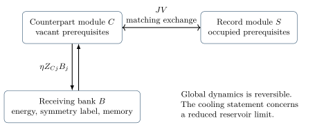
5.3 How the cold response follows from the bank state
The vacuum correlation in the supplied Hamiltonian parameter is
Assume the weak-coupling, secular reservoir limit, with at fixed . This is the setting of quantum Markovian reservoir theory [8]; we analyse the resulting finite generator, without claiming a finite- convergence bound for the microscopic model. Let be full eigenspace projectors of the interacting . Define
5.4 A convergence criterion, and its verified domain
Dissipation into a dark target is not sufficient for preparation if other dark subspaces remain [9]. Engineered dissipation as a resource for state preparation is established prior art [10]. Here the question is whether the stated bank source supplies the required transitions. For each excited eigenspace define its downward escape operator
Proposition 5.2 (Conditional preparation in the limit generator). Suppose has a unique ground state and every excited is strictly positive on its eigenspace. Then (36) converges to that ground state from every initial density matrix.
Proof. Using gives
The minimum level spacing in this proof is not the ground gap. An early numerical bound used the latter in its place; that field is retained as an error in the evidence, and only the corrected bound is used here.
For the six declared cases and , all 64 system energy levels are simple and every excited escape rate is positive. The evaluated generators therefore satisfy the criterion. At their ground state is ; at they cool to a different state. The source repairs preparation conditional on the prior selection mechanism; it does not derive the required exchange hierarchy.
For these simple spectra, order populations by energy. The cold population generator is triangular with diagonal , where is the total downward rate. Its spectral gap is . For coherences,
| Population gap | Full quantum gap | |
|---|---|---|
| 2 | ||
| 8 |
These are rates in , not physical times at a verified finite coupling. An initial state’s population convergence can be faster than the slowest mode; a gap alone is not a complete finite-time error bound. The tested nine-input population times to reach about in slow units. Broader sampled parameter scans do not prove an interval theorem for every .
5.5 Where energy and quantum information go
The exact microscopic conserved energy is . The reduced generator keeps the leading reservoir-limit energy exchange; it is not an exact finite-coupling energy ledger. To see the memory requirement without hiding unsuccessful routes, put and choose . The map
This dilation exhibits the retained output information. It does not prove that a finite autonomous bank implements an indefinite sequence of fresh outputs. If 64 mutually orthogonal inputs all give the same pure state, reversibility requires their orthogonality to move into at least 64 distinguishable bank states. A maximally mixed input exports six bits of entropy; an input entangled with a reference requires preserving six qubits of quantum information. Cooling cannot be credited as a free reset or a clone of an input.
5.6 Spectral regularity and finite-coupling dressing
The cold spectrum cannot be altered solely to accelerate the reduced equation without checking the microscopic energy. Completing the square in (31) gives
For the broader assumed spectral family
The preparation result consequently assumes an initially cold continuous reservoir, distinguishable read types, weak coupling, secular resolution and unlimited retained history in the limiting description. None is supplied by the finite clock construction. A finite bank that prepares the clock before appreciable return, with controlled errors and all memory retained, remains unconstructed.
6 Coherent storage and its response
6.1 A budget per configuration
Consider interchangeable two-state storage entries. Their labels carry no spatial location. Let denote a definite occupied subset with . The adopted push rule is
Let be the normalised uniform sum of all subsets. Each target subset of size has predecessors. Thus its amplitude after the push is . Using gives
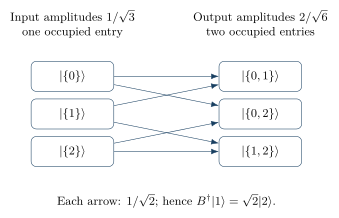
Writing and for occupation,
A constant-amplitude ladder instead has in its interior. Last-in, first-out ordering does not require constant amplitudes: a stack could be given the square-root law as an additional input. Hence the result does not prove that any-order access is necessary. Its merit here is that the chosen matrix elements follow from the stated configuration rule and route counting.
6.2 An exactly soluble single-record comparison
To separate a ladder effect from the more complex transaction energy, first take a distinct calibration action,
Equation (53) also fixes the sign for this calibration model: for and the square-root interior ladder, the filled record reduces the gap exactly when . The storage law does not fix that energy ordering. These dressed spectral gaps require a specified readout before they become an operational clock comparison; the next construction supplies one.
7 Response to the full transaction energy
7.1 The action and the controlled reduction
Attach the finite occupation bank (49) to the full source (3):
Take greater than the source bandwidth and sufficiently small that adjacent bank-number bands remain isolated. The explicit form of in (3) gives by the triangle inequality, since each and has norm one. Thus, for the tested , the bandwidth is at most , below both tested bank spacings . In an energy basis, second-order block elimination gives
For adjacent interior steps of the square-root ladder,
7.2 A readout of the reduced response
Let embed the bare source at occupation , and let be the exact projector onto the isolated interacting band continued from it. The positive-overlap isometry
In the registered tests, the exact reduced and full-Hamiltonian coherences agree to over the declared probes. Substitution of bare, undressed coherences fails the control. Capacity was compared with on two interior responses; the exact matrices changed by at most . These are finite convergence checks, not an unlimited-capacity theorem.
7.3 The positive free-record identity
The stationary response is the complete energy-block-diagonal part
Proposition 7.1 (Free records at second order). For independent records with , and , the formal stationary same-occupation coefficient is
Proof. Decompose into Bohr components, . There are only . In the eigenbasis for one record,
Thus the stationary response is exactly energy-proportional at second order, for any finite number of independent records. For positive the coefficient is negative precisely when , the single-record transition energy in these units. Higher source energy then reduces the probe frequency at this order. Neither packet conservation nor configuration-wise normalisation fixes this ordering. At finite higher-order corrections remain.
One-step denominators alone do not establish an isolated clock. At a two-packet resonance mixes occupations already at order , even though the denominators at are avoided. At , two free records have a third-order resonant path, with a competing second-order diagonal splitting. Appendix B gives both blocks. A divergent perturbative expression at resonance is a failure of the reduction, not a divergence of the finite Hermitian Hamiltonian or proof that no clock can exist.
7.4 The interacting module fails the energy-only test
For a source eigenstate , the response is
For and , Table 3 shows three energy-paired comparisons. The members of each pair have identical packet-count distributions, because word parity maps one eigenstate to its opposite-energy partner without changing word probabilities. Nevertheless the response-to-energy slopes differ by a factor of approximately . A single coefficient cannot describe them.
| Source energies | Coefficients | |
|---|---|---|
The mechanism can be made explicit. For (3), . In a real energy eigenbasis, gives off the diagonal, and the commutator gives . Substitution in (67) yields
A larger bank quantum does not repair the leading relative discrepancy. Put and . Expanding the denominators gives
Since , has zero block-diagonal part in the eigenspaces. If were proportional to , every ratio
The tested alternatives with other interaction gates also fail the stationary energy-only diagnostic. The scope is those specified actions and readouts. The calculation is not a theorem that all interactions or all possible dressed observables must fail.
8 Testing the counterpart clock itself
The occupation probe above is an added construction. It is therefore important to test the unchanged counterpart clock (20), rather than assuming the two probes are interchangeable.
8.1 The selected-state reading has no extra rate
Equation (25) is independent of , while the full state’s eigenvalue changes from to . For that state and that reading, exchange changes the global energy but does not generate an additional energy-dependent conditional rate. This exact zero is specific to the stated conditional observable. It does not exclude every alternative dressed clock.
8.2 A loaded clock can detect equal-energy coherence
A second experiment prepares a source eigenstate and a clock coherence between distinct clock energies. This disturbs the selected state and is a different preparation. At , partial tracing the full commutator gives the exact clock generator , with
There is a particularly simple counterexample. Let integer word labels use bit 0 as the least significant bit, and set
This witness concerns the native matching exchange, whose third-label transfer is ungated. The occupation probe in (55) instead couples through the gated . The difference is physical and stated, not a change of notation. Even three free records fail the energy-only test for the native loaded readout: a source with signs gives , so equal clock gaps associated with labels 0 and 2 have opposite fractional shifts. This does not contradict (63), which concerns a different bank action, reduction and observable.
An explicitly supplied energy-product interaction can pass the desired diagnostic. That is a useful positive control for the measurement, but inserting it would assume the property under investigation. No such replacement is made in either negative result.
9 Relation to prior work and the remaining problem
9.1 What the construction inherits
Relational time in a stationary quantum state is the Page–Wootters proposal [1]. The conditioning and measurement-accounting framework used here belongs to its subsequent development [2]. Results about factorisation, clock ambiguity and equivalence between relational descriptions have stated assumptions about clocks, constraints and subsystem structure [3, 15]. Our counterpart rule specifies a factorisation and an action; it does not prove uniqueness of that choice.
Finite clocks introduce spectral compatibility, measurement resolution and periodicity issues [4–6]. Section 3 supplies an example in which improving a fixed-window approximation does not give exact stationarity or full-period convergence. A clock-dependent conditional state, an external diagnostic-time frequency, and a physical observer’s reading remain distinct objects.
The state (21) is maximally entangled under a local mirror transformation. At inverse temperature , the thermofield double
The storage amplitudes implement the known Dicke and Holstein–Primakoff algebra [11–13]. Their interpretation as a configuration-normalised bank rule exposes the resource premise; it does not derive bosonic statistics from nonquantum assumptions. The cold limit uses established dissipative preparation methods [8–10], and its finite-bank extension remains open.
9.2 Comparison with assumed gravitational clock couplings
Interactions between a clock and a system generally change conditional evolution; they need not reduce to a scalar rate change. Smith and Ahmadi derive a general interacting-clock conditional kernel [16]. Their gravitational example starts from an energy-product coupling with a supplied distance and gravitational constant. Castro Ruiz, Giacomini and Brukner analyse the implications of
A close comparison is Singh and Friedrich [18]. Their constraint includes the explicit product
Cafasso and collaborators specify pairwise clock-energy products and coupling constants before deriving interaction transfer [19]. The clock calculations in chapter 7 of Favalli’s treatment use specified gravitational potentials or their relativistic counterparts [20]. These inputs are appropriate to those questions. They do not derive distance, universal coupling or its coefficient from the record transactions studied here.
The difference is precise. An assumed interaction is energy-only by construction. Equation (67) instead sums matrix elements of transaction operators. The free-record identity shows that this sum can collapse to total energy. The counterexamples show why that collapse cannot simply be assumed to survive interactions or a change of observable.
9.3 Why a negative frequency shift is not yet gravity
No distance or operational spatial relation has been derived, so there is no inverse-distance potential, field propagation law, tidal observable or gravitational constant to compare with experiment. The energy-centred coefficient also does not assign an absolute gravitational role to an arbitrary additive constant in a finite Hamiltonian.
Quantum formulations of the equivalence principle distinguish rest, inertial and gravitational energy operators. Agreement of selected diagonal expectations is weaker than equality of those operators [21]. The free stationary identity is therefore a limited positive result, not the equivalence principle. Established scattering arguments for universal gravitational coupling use relativistic and massless-spin-two assumptions absent here [22]; importing their conclusion would not derive those assumptions from records.
The three binary labels are not three physical generations. They define a finite test module. Its gated interaction has not produced a proton, a field-theoretic scattering amplitude or a measured mass ratio. Such claims require additional derivations and an observable map. No empirical particle data enters any coefficient reported here.
9.4 A focused requirement for further progress
For preparation, the bank must receive every obstructing conserved label as well as energy, and its low-entropy acceptance resource and retained memory must be explained. For a universal stationary clock response, a transaction law must imply a relation of the form
Increasing the capacity of an unchanged source or fitting a coefficient to each eigenstate does not meet these requirements. A successor must state an interaction or symmetry and show why it enforces the identity. A finite preparation model with complete energy and memory accounting would also be useful even without universal energy response. The construction remains a rigorous pedagogical example in that case.
10 Conclusions
A vacancy counterpart of a finite record rule generates complementary energies, and matching exchange selects a state supporting exact conditional evolution. This reduces the independently specified clock data, while leaving the counterpart rule and exchange hierarchy as assumptions. Closed evolution does not prepare the selected eigenstate. A finite receiving bank exposes a symmetry obstruction; a source that exports the label permits conditional preparation in a cold continuous-reservoir limit.
Configuration-wise normalisation gives a truncated bosonic ladder. Its dispersive coupling to independent records has a stationary second-order response proportional to energy, with a sign determined by the energy ordering. The tested gated records violate that proportionality, including in the leading large-frequency coefficient. The native counterpart clock gives an exact equal-energy counterexample under a different readout.
The work establishes explicit models, derivations and reproducible limitations, not a physical vacuum substrate or emergent spacetime. Compatible energies, selected correlations, preparation, access and universal energy response are separate demands on a transaction rule. The missing implication can now be stated and tested mathematically.
Computational practice and availability
All numerical results come from retained finite-model packages and separately implemented reviews. The evidence was consolidated in M5 after clean exports of committed source trees were replayed. Baselines, deliberate faults, original failures and corrections are mapped in Appendix C. A successful implementation check is not empirical validation; two implementations of one model are not two physical observations.
The supporting code, numerical data, registrations, corrections and implementation reviews are archived on Zenodo [23]. The cited concept DOI identifies the evolving collection; the exact evidence release used here is version 1.0.0, doi:10.5281/zenodo.24109717. It includes portable replay commands and a distribution manifest. Scientific sources and saved results are unchanged from the frozen evidence commit. Third-party article texts, private coordination logs and the administrative database are excluded. The paper’s separate Zenodo record contains this PDF and editable LaTeX source, including build instructions and the evidence map.
Acknowledgements and disclosure
The research and manuscript were developed with assistance from Codex and Claude for algebra, programming, cross-checking, literature retrieval and drafting. Their separately constructed implementations and critiques are recorded. This process is computational verification, not independent experimental confirmation or journal peer review. David Elliman is the author; the author approved this preprint and its archival release.
A Spectrum of the three-record module
The explicit form in (3) shows that for every . For the spectrum quoted here set and work in the eigenvalue sector . On the other two bits, . The antisymmetric vector has eigenvalue zero. In the remaining symmetric basis ,
For , and even integer , exact matching to the uniform clock requires , a rational number. Only can occur. The exact shell therefore contains only the two dark source modes at energy three and a single clock level . It cannot represent nontrivial source dynamics. This is a limitation of this rational uniform-clock family, not of every finite relational clock.
B Resonances and the order of the response
The same-occupation coefficient in (63) cannot discard other states degenerate with its chosen band. The examples here use finite occupation states and the same free-record action, without spatial interpretation.
B.1 A second-order two-packet resonance
For one free record, , the energies of and are two and zero. At , and have equal unperturbed energy. The first direct matrix element vanishes, but two transactions connect them. For the full second-order block is
Diagonal splitting and mixing in (84) have the same order. The largest limiting bare-state weight is
At first and second order, positive cross-occupation free-record resonances occur at or : one or two transactions change source energy in multiples of two while changing occupation by one or two. Zero frequency is singular; same-occupation source degeneracies also remain. This is not an all-orders exclusion of other resonances.
B.2 A third-order path at
For two free records, and have common energy at . Retaining the pair gives
| Bank changes | Path sum |
|---|---|
Their sum is ; normalising occupation states multiplies it by . Thus the coefficient is derived without fitting a level splitting.
The second-order separation is , so mixing at fixed is only and vanishes in the limit, unlike (84). The leading avoided-crossing centre and gap are
C Reproducibility, corrections and claim provenance
C.1 What was replayed
Scientific implementations use Python, NumPy and SciPy, with no imports from previous spatial-lattice code. The original environment was Python 3.13.7, NumPy 2.4.4 and SciPy 1.17.1, with single-threaded BLAS. Complete finite spaces, reverse routes and named memory factors are retained. Reductions, limits and supplied measurements are identified explicitly.
The constructor evidence tree is 84122c9; the review tree was replayed at 97dfae2. The constructor replay record is committed at df0ddca. Clean git archive exports isolate calculations from uncommitted files. A pristine copy is retained separately from the execution copy, including for scripts that use fixed output names.
Constructor-side consolidation reproduces 32 main processes: ten baselines with exit zero and 22 faults with exit one. Eight additional processes reproduce post-hoc checks and their faults; original M3’s accuracy failure also replays with exit one. Scientific JSON values agree at absolute/relative tolerance , numeric arrays at the same tolerance, and text arrays exactly. Runtime, timestamps and resource-use fields are excluded explicitly. All 980 pristine files match their committed Git blobs afterwards. A separate reviewer replay of three constructor baselines and five cross-package comparisons agrees. These establish reproducibility on the stated environment, not statistical significance or physical truth.
Three mistakes in the replay harness were retained and corrected: treating text-array labels as numbers, omitting a runtime-field spelling and using a CLI fault name instead of its saved directory alias. A review-side comparison initially differed only in its exit-footer format. No scientific source or tolerance changed. The supporting archive retains these logs.
C.2 Evidence units and corrections
Quoted error bounds are rounded upward at their stated precision; central estimates are rounded to the nearest stated digit.
Unit identifiers in Table 4 are reproducibility labels. The companion EVIDENCE.md gives full directories, result paths and commands.
| Unit | Claim used here | Scope or correction retained |
|---|---|---|
| Unit | Claim used here | Scope or correction retained |
| PW1 | Finite-clock bound and benchmark; stationary matched spectrum | Fixed-window convergence only. Instrument error is an upper bound. |
| PW2 | Counterpart identity; selected eigenstate and threshold; gap from M3b | Matched strengths and hierarchy assumed; readout efficiency is family dependent. |
| PW3 | Finite-bank failure and sector obstruction | Nine word inputs; four sector-admissible review inputs also fail in the sampled window. Symmetry proof is post hoc. |
| PW4 | Cold response, label export, escape criterion, memory | Reservoir limit; level-spacing bound corrected; full decay gap is half the population gap. |
| M2 | Storage rule, finite ladder and two-state blocks | Budget per configuration; interior uniformity at second order; LIFO not ruled out. |
| M3 | Dispersive response, dressed readout and interacting mismatch | Original six accuracy failures retained; refinement at unchanged tolerance. Moment obstruction is post hoc. |
| M3b | Native conditional zero and equal-energy witness | Two readouts; initial derivative is not a persistent late-time rate. |
| M4 | Free-record sign and resonant corrections | Original two accuracy failures retained. Extrapolation tests a limiting coefficient. Third-order follow-up separately checked. |
| M0 | Literature and exact prior-art identifications | metadata checks; eight priority comparisons independently checked at equation level. |
M3’s original checks missed a spectral bar in six cases. The recorded amendment added , retaining the action, original samples and tolerance; the finest error is at most . M4’s original Richardson pair missed its coefficient-accuracy bar twice at . The declared replacement pair passes the same bar, with worst relative error . Extrapolation estimates a coefficient, not an exact finite- equality. The failed outputs are preserved.
PW4’s baseline field energy_decay_bound used the ground gap instead of the minimum level spacing. It is not used here as a valid bound. The corrected coefficient, population/coherence distinction and low-energy spectral qualification are explicit. A sampled search for dark states or crossings is not a proof for every real coupling.
C.3 Reference verification
The bibliography contains 22 published works whose DOI metadata were checked against publisher/Crossref records and available primary manuscripts. Detailed comparisons with Smith–Ahmadi, Singh–Friedrich, Cafasso and collaborators, Castro Ruiz and collaborators, Cottrell and collaborators, Emary–Brandes, Favalli’s chapter 7 and Chataignier and collaborators were also checked separately at equation level. The selected-state and finite-ladder identifications were instantiated algebraically.
Full text of the original Page–Wootters and Holstein–Primakoff articles was unavailable in the recorded retrieval; Davies and Weinberg were used at contextual abstract/metadata scope. Their detailed mathematical roles here are either derived explicitly or supported by accessible primary sources cited alongside them. Favalli’s book was read selectively, not in full. These limits are recorded, and no priority claim is inferred from the search. The additional Verstraete–Wolf–Cirac citation was checked against publisher-deposited metadata and the authors’ manuscript for its dissipative-preparation claim; its lattice constructions are not imported into this model.
The supporting-software entry was verified against its published Zenodo record; it identifies the exact version used and the concept DOI for the collection.
References
- Don N. Page and William K. Wootters. Evolution without evolution: Dynamics described by stationary observables. Physical Review D, 27: 2885–2892, 1983. doi:10.1103/PhysRevD.27.2885.
- Vittorio Giovannetti, Seth Lloyd, and Lorenzo Maccone. Quantum time. Physical Review D, 92: 045033, 2015. doi:10.1103/PhysRevD.92.045033.
- Philipp A. Höhn, Alexander R. H. Smith, and Maximilian P. E. Lock. Trinity of relational quantum dynamics. Physical Review D, 104: 066001, 2021. doi:10.1103/PhysRevD.104.066001.
- Tommaso Favalli and Augusto Smerzi. Time Observables in a Timeless Universe. Quantum, 4: 354, 2020. doi:10.22331/q-2020-10-29-354.
- Mischa P. Woods, Ralph Silva, and Jonathan Oppenheim. Autonomous Quantum Machines and Finite-Sized Clocks. Annales Henri Poincaré, 20: 125–218, 2019. doi:10.1007/s00023-018-0736-9.
- Leonardo Chataignier, Philipp A Höhn, Maximilian P E Lock, and Fabio M Mele. Relational dynamics with periodic clocks. New Journal of Physics, 28: 034504, 2026. doi:10.1088/1367-2630/ae46d0.
- William Cottrell, Ben Freivogel, Diego M. Hofman, and Sagar F. Lokhande. How to build the thermofield double state. Journal of High Energy Physics, 02: 058, 2019. doi:10.1007/JHEP02(2019)058.
- E. B. Davies. Markovian master equations. Communications in Mathematical Physics, 39: 91–110, 1974. doi:10.1007/BF01608389.
- B. Kraus, H. P. Büchler, S. Diehl, A. Kantian, A. Micheli, and P. Zoller. Preparation of entangled states by quantum Markov processes. Physical Review A, 78: 042307, 2008. doi:10.1103/PhysRevA.78.042307.
- Frank Verstraete, Michael M. Wolf, and J. Ignacio Cirac. Quantum computation and quantum-state engineering driven by dissipation. Nature Physics, 5 (9): 633–636, 2009. doi:10.1038/nphys1342.
- R. H. Dicke. Coherence in Spontaneous Radiation Processes. Physical Review, 93: 99–110, 1954. doi:10.1103/PhysRev.93.99.
- T. Holstein and H. Primakoff. Field Dependence of the Intrinsic Domain Magnetization of a Ferromagnet. Physical Review, 58: 1098–1113, 1940. doi:10.1103/PhysRev.58.1098.
- Clive Emary and Tobias Brandes. Chaos and the quantum phase transition in the Dicke model. Physical Review E, 67: 066203, 2003. doi:10.1103/PhysRevE.67.066203.
- Sergey Bravyi, David P. DiVincenzo, and Daniel Loss. Schrieffer–Wolff transformation for quantum many-body systems. Annals of Physics, 326: 2793–2826, 2011. doi:10.1016/j.aop.2011.06.004.
- Chiara Marletto and Vlatko Vedral. Evolution without evolution, and without ambiguities. Physical Review D, 95: 043510, 2017. doi:10.1103/PhysRevD.95.043510.
- Alexander R. H. Smith and Mehdi Ahmadi. Quantizing time: Interacting clocks and systems. Quantum, 3: 160, 2019. doi:10.22331/q-2019-07-08-160.
- Esteban Castro Ruiz, Flaminia Giacomini, and Časlav Brukner. Entanglement of quantum clocks through gravity. Proceedings of the National Academy of Sciences, 114: E2303, 2017. doi:10.1073/pnas.1616427114.
- Ashmeet Singh and Oliver Friedrich. Emergence of Gravitational Potential and Time Dilation from Non-interacting Systems Coupled to a Global Quantum Clock. Foundations of Physics, 55: 82, 2025. doi:10.1007/s10701-025-00893-8.
- Dario Cafasso, Nicola Pranzini, Jorge Yago Malo, Vittorio Giovannetti, and Marilù Chiofalo. Quantum time and the time-dilation induced interaction transfer mechanism. Physical Review D, 110: 106014, 2024. doi:10.1103/PhysRevD.110.106014.
- Tommaso Favalli. On the Emergence of Time and Space in Closed Quantum Systems. Springer Theses. Springer, 2024. doi:10.1007/978-3-031-52352-6.
- Magdalena Zych and Časlav Brukner. Quantum formulation of the Einstein equivalence principle. Nature Physics, 14: 1027–1031, 2018. doi:10.1038/s41567-018-0197-6.
- Steven Weinberg. Photons and gravitons in S-matrix theory: Derivation of charge conservation and equality of gravitational and inertial mass. Physical Review, 135: B1049, 1964. doi:10.1103/PhysRev.135.B1049.
- David Elliman. Supporting code and evidence for relational clocks in a quantum ledger, 2026. URL https://doi.org/10.5281/zenodo.24109717. Version 1.0.0. Concept DOI: 10.5281/zenodo.24109716. The URL above identifies the exact version.
The version of record is archived on Zenodo at the DOI above; this page and PDF are the publisher copies at neusym.ai. See the full list of papers for the rest of the programme.