In general relativity, clocks, moving matter and light all respond to one common spacetime geometry. Can small quantum networks reproduce part of that agreement? We study several finite models, and separate what is calculated from the assumptions about gravity that are put in by hand. The strongest result is a controlled test of how probes read a supplied smooth geometry. One lattice version of the Dirac equation (the relativistic wave equation for spin-one-half particles) governs a clock and both massive and massless wave packets. Lattice spacing, how quickly the field varies, packet width and box size are varied separately, without fitting the readouts. Exact response formulas and Taylor-expansion bounds give explicit errors. In the smoothest field, the clock–speed relation is enclosed within about one percent of its reference value. The ratio of the field gradients inferred from forces on massless and massive packets lies in [1.9399, 2.0619], around the prescribed value two. Keeping the sign of second-order contributions sharpens this force bound without assuming perfect symmetry. A simpler local lattice law also approximates the full evolution of the prepared packet, with state-vector error bounded by 0.004612 over the tested time window. A separate calculation with a trapped source shows a delayed arrival over several lattice sites and an inward displacement, but its geometry readout remains less well controlled. Other models retain coherent transport by a colour clock, entanglement generated through a quantum mediator, and exact relations between entanglement entropy and graph cuts. These constructions are not yet one microscopic theory. The results provide reproducible benchmarks for recovering a geometry, rather than a derivation of gravity. The stresses that hold the source together, universal coupling, a continuum limit with a spatially varying field, and dynamical gravitational equations remain open. The paper supplies the error analysis needed to distinguish promising finite-model behaviour from those stronger claims.
Elliman, D. (2026). Quantum Clocks and Geometry: Gravity-inspired tests in finite quantum networks. Neuro-Symbolic Ltd technical report. https://doi.org/10.5281/zenodo.23987420
@techreport{elliman2026qutritgravity,
  author      = {Elliman, David},
  title       = {Quantum Clocks and Geometry: Gravity-inspired tests in finite quantum networks},
  institution = {Neuro-Symbolic Ltd},
  year        = {2026},
  doi         = {10.5281/zenodo.23987420},
  url         = {https://neusym.ai/papers/qutrit_gravity/}
}
Full text
The complete paper, rendered as HTML with the mathematics set at build time. The PDF above is the typeset version
of record; equation, theorem and reference numbers match it.
1 The question and the level of evidence
Gravity is measured through relationships between physical systems: how clocks compare, how bodies move, and how light propagates. This suggests a concrete question for a quantum-network model. Can one microscopic law make these different measurements agree on a common effective geometry? In general relativity they agree automatically, because all of them read the same spacetime metric. In a model built from quantum registers that agreement has to be demonstrated rather than assumed.
The calculations in this paper test ingredients of such a programme. They do not yet answer that question for a single law. It helps to keep the four constructions apart from the start. The colour clock, the scalar and two-potential fields, the spin mediator and the entanglement network are distinct constructions. Their Hilbert spaces and Hamiltonians are specified separately. Sharing qutrit registers or a graph does not by itself connect their dynamics.
A qutrit is a quantum system with three basis states, the three-level analogue of a qubit. Here, “colour” means a three-dimensional representation of SU(3), the symmetry group that rotates those states. (A representation is a rule assigning a matrix to each symmetry operation.) The word is borrowed from the strong interaction, but using it does not establish quantum chromodynamics. Likewise, a register that oscillates can serve as a clock without being a physical atomic clock. These distinctions let us investigate small, exactly specified systems while keeping their physical interpretation proportionate to the evidence.
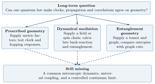
Figure 1. The three lines of investigation. Dashed arrows indicate work still required, not established implications.
Because the paper mixes exact algebra, numerical experiments and physical interpretation, we label which kind of claim is being made. We use three kinds of statement. An operator identity follows from the finite matrices and can be exact. A numerical result refers to specified parameters, initial states and readout times. A physical interpretation requires additional assumptions, such as identifying a supplied scalar with a gravitational potential. Passing a numerical check does not supply those assumptions.
The colour-transport construction extends the pairing-algebra analysis of Ref. [1]. Section 2 introduces only the algebra needed to understand its clock readout; Appendix A gives the detailed reduction. Sections 3 and 4 examine prescribed geometry and scalar back-reaction. Section 5 adds the earlier two-potential source calculation and distinguishes its local readouts from propagation. Section 6 introduces a common-regulator Dirac model and a multi-site arrival experiment. Section 7 then separates lattice, packet, field and boundary effects and derives explicit readout and finite-time error bounds for a smooth reference geometry. Section 8 studies a genuinely quantum mediator (a quantum system that carries an interaction between two probes). Section 9 then asks a different, kinematic question about entanglement and graph cuts. Readers who want the most controlled result can go directly to Section 7.
We use ℏ=1 and model units, so energies and inverse times are measured in the same unit. The reference light speed is one in the continuum metric formulas; numerical lattice speeds and spacings are stated explicitly in each experiment. Couplings are not measured masses or gravitational constants. Clock parameters are calibrated; Appendix I specifies the computational evidence and its scope.
2 A colour clock built from entangled pairs
2.1 Why pairing replaces swapping
The first ingredient is a clock that transports colour information. The idea is that the clock’s “ticking” moves a colour label from one end of a small register chain to the other, so that the clock’s rate could later be compared with other processes. Its internal cluster consists of eight fundamental colour qutrits (qutrits that transform as the basic three-dimensional representation 3). A sum of pair exchanges selects a low-energy sector that transforms as an antitriplet, 3ˉ, under SU(3). Two external registers, A and C, remain fundamental triplets. The relevant colour space is therefore
Hcol=3A⊗3ˉB⊗3C.(1)
Here B labels the collective colour of the cluster, not an additional physical qutrit. A triplet and an antitriplet transform differently, roughly as a vector and its complex conjugate do. Swapping their labels is therefore not the invariant operation that a fundamental–fundamental exchange would suggest.
The natural invariant instead asks whether a triplet and antitriplet form a colour singlet, a combined state that is unchanged by every colour rotation. For the pair BX, with X=A or C, define
The factor of three appears because Ω is not normalized. Thus K2=3K: it is three times a projector, not a swap. The two contractions obey
KABKBCKAB=KAB,KBCKABKBC=KBC.(3)
These are Temperley–Lieb relations with loop weight three [2]. They reduce the colour dynamics to a small pairing space: all that matters is which pair currently forms the singlet.
For each total colour c, two useful normalized states are
They describe the same total colour carried by different pairings. Their overlap is 1/3, so they are not orthogonal alternatives. A transfer experiment includes distinct initial and final clock states as well as these colour states; the quoted transfer probability concerns that full specified target.
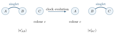
Figure 2. Singlet handoff changes which pair stores the singlet and which end carries the total colour. The diagram depicts relationships between registers, not physical distances.
2.2 The spectator amplitudes must remain coherent
Not every colour state takes part in the singlet handoff. The colour space separates into a six-dimensional active sector, which the contractions act on, and a twenty-one-dimensional spectator sector, which they leave alone:
Hcol≅(3⊗C2)⊕6ˉ⊕15.(5)
Both contractions annihilate the last two sectors. A Hamiltonian built only from the identity and these contractions acts identically on their colour labels, although the internal clock may still evolve. An uncontracted colour basis state generally has components in both sectors. Their amplitudes must be added before taking the squared modulus, as in any interference experiment. Dropping the spectator term changes the experiment.
For the particular colour basis transition ∣0,0ˉ,2⟩→∣2,1ˉ,1⟩, the active weights are each 3/8 and the spectator overlap is 1/8. The resulting bounds are
The first bound applies when the spectator transition amplitude vanishes or is excluded. The second retains its coherent contribution. Neither is a bound on arbitrary SU(3)-invariant dynamics: a larger invariant algebra can distinguish spectator irreducible representations. Appendix A supplies the derivation.
2.3 Calibrated transport with a finite selection gap
We now turn the algebra into a working clock. A port is the set of pair exchanges that couples the cluster to an external register. Projecting a physical exchange port into the selected cluster sector gives an internal clock operator Ma multiplied by I/6−K/2. Adding a specified internal term changes that colour factor into a reflection:
R reverses the sign of the singlet and leaves the octet unchanged. It is Hermitian and unitary. The two such reflections do not obey the permutation braid relation, so an old permutation calibration cannot simply be reused.
The revised model solves algebraic conditions on seventeen internal coefficients and adds finite-gap counterterms (extra terms that compensate for the energy shifts caused by brief excursions out of the selected low-energy sector). Its reference clock states are dressed: about 6.85% of their weight lies outside the simplest bare clock subspace. Table 1 summarizes the retained numerical benchmark, at the fixed readout time tπ=256,000π.
Table 1. Calibrated clock–colour transfer. The finite-gap calculation retains virtual excursions into additional cluster representations, within a fixed total-fundamental colour sector. It does not test arbitrary coherent superpositions of all total-colour sectors. Values are rounded from the existing independently replayed clock records.
Calculation
Singlet-target probability
Omitted-sector leakage
Projected, 84 multiplicity states
0.999809
excluded by projection
Finite gap Δ8=25,600, 210 states
0.916935
1.07×10⁻⁷
Finite gap Δ8=102,400, 210 states
0.995818
6.72×10⁻⁹
Here leakage is the probability found outside the intended sector at the readout time. Small leakage does not guarantee small dynamical error. A tiny virtual energy shift can accumulate a substantial phase over the long readout time. At the smaller gap, transfer is only 91.69% despite leakage near 10−7. At the larger gap it reaches 99.58%, but removing the external counterterm lowers it to 87.48%. Finite-gap returns and calibration are therefore part of the result, not negligible details. None of these figures establishes a naturally selected clock, a fermion, or gravitational protection of its energy levels.
3 What it means to supply a geometry
3.1 Clock rate, spatial scale and shift
This section asks what can be learned by supplying a geometry by hand and checking how clocks and hopping respond to it. A spacetime metric tells us how coordinate intervals relate to measurements by clocks and rulers. We use the ADM convention [3], which splits spacetime into a sequence of spatial slices,
ds2=−N2dt2+hij(dxi+βidt)(dxj+βjdt).(8)
The lapse N relates coordinate time to the proper time of observers normal to a spatial slice. The shift βi relates the spatial coordinate grids on neighbouring slices. For a static isotropic metric with zero shift, write
hij=n2δij,N=eϕ,n=e−ψ.(9)
Here ϕ and ψ are logarithmic potentials: ϕ<0 means clocks run slow. A stationary clock then has dτ=Ndt and a coordinate light ray has speed N/n. The scalar prescription ψ=ϕ makes this speed e2ϕ; that equality is a chosen model rule, not an exact identity for every general-relativistic metric.
For constant N, multiplying an entire Hamiltonian by N gives
e−itNH0=e−iτH0,τ=Nt.(10)
Every transition therefore reaches the same probability at a coordinate time enlarged by 1/N: a clock with N<1 simply runs slow. This is an exact time-rescaling identity. It is a useful consistency test of a clock implementation, but cannot derive gravitational redshift: the multiplier has already supplied it.
The existing clock records pass this uniform-lapse test. (A Ramsey readout measures a clock’s frequency from the phase it accumulates between two pulses.) In one declared scalar well, a lapse near 0.972640 gives Ramsey readouts near 0.972679 in the projected clock and 0.972643 in the finite-gap clock. Nonuniform weights also change the transfer fidelity. Such changes are responses to a specified gradient. A first spatial gradient is not, by itself, an invariant tidal curvature; testing tidal gravity requires a metric, connection and curvature comparison.
3.2 Virtual hopping exposes an assumption in the coupling rule
A low-energy hop can proceed through intermediate excited states: the system briefly visits a higher-energy state and returns. In second-order perturbation theory, its scale is roughly hopping amplitude squared divided by the excitation energy. More precisely, with P the low-energy projector, Q=I−P, hop V and positive excited-state operator D, define
Θ=PVQ(QDQ)−1QVP.(11)
Θ is positive semidefinite. For an unperturbed low-energy eigenvalue chosen as zero, the corresponding second-order Hamiltonian correction is −Θ[4]. Evaluating the inverse exactly does not make this expression an all-orders effective Hamiltonian.
Suppose a prescribed geometry changes V by N/n. We would like the effective hop Θ to slow down with the clocks, that is, to scale as N. That requires the relevant denominator to scale as N/n2, within this common-scalar weighting ansatz:
Θ(N,n)=N/n2(N/n)2Θ(1,1)=NΘ(1,1).(12)
The cancellation is exact at this perturbative order for all positive N,n. It is an engineered compatibility condition. Other microscopic couplings could realize the same readout differently.
The next example shows how this choice of denominator plays out in a concrete model. The finite gauge-register model distinguishes a one-link virtual dipole (a short-lived pair of opposite charges on neighbouring sites) from a longer open string. Let ΠE project onto an excited electric link and ΠZ,f,ΠZ,g onto charged endpoint syndromes (the local checks that detect a charge at each end). Define
Pdip=ΠEΠZ,fΠZ,g,Pflux=ΠE−Pdip.(13)
These are orthogonal and commute with the declared discrete Gauss generators. A one-link hop from the vacuum charges both ends and activates Pdip. Extending the string by one link neutralizes the middle register; neither of its two links then has two charged endpoints. Both activate Pflux. This is a statement about these configurations, not a classification of every possible many-charge state.
Giving the face and dipole gaps the common factor N/n2 produces Eq. (12). The alternative unsplit penalty ΔENn gives
Θunsplit∝2ΔZ+ΔEn3J02N,(14)
which retains a dependence on n. The numerical failure of pure-lapse scaling is thus predictable directly from the denominator.
There is a separate physical distinction here. The Maxwell Hamiltonian at fixed canonical electric flux has metric weight N/n in three isotropic spatial dimensions:
HE=21∫d3xhNhijπiπj=21∫d3xnNδijπiπj.(15)
Writing an energy in terms of a covariant electric field instead can display Nn, but that holds a different variable fixed. The qutrit’s discrete flux label has not been derived as either continuum variable. Its Nn flux penalty is therefore retained only as a supplied rule, not identified with the canonical Maxwell flux energy.
3.3 A local dispersion test is not a curved-space field theory
This subsection checks how far a supplied metric can be built into a Dirac-type lattice Hamiltonian, the standard description of relativistic spin-one-half matter. Let constant matrices Γ0,Γa obey the Dirac Clifford algebra, and let a spatial frame eai satisfy ∑aeaieaj=hij. Setting γi=∑aeaiΓa gives {γi,γj}=2hijI. At a point where the coefficients are frozen, the lattice Hamiltonian consistent with Eq. (8) is
H=N(i∑γipi+mΓ0)−βipiI,pi=J0sinki.(16)
In particular,
(H+βipiI)2=N2(hijpipj+m2)I.(17)
In words: apart from the shift term, the squared energy has the relativistic form “momentum squared plus mass squared”, with the local metric and lapse inserted; pi approaches the ordinary momentum when ki is small. The minus sign of the shift follows from the metric convention. The original code uses a plus-sign shift coefficient; its coefficient is −βi in our notation.
This construction spans all six components of a symmetric spatial metric and reproduces the local relativistic mass shell at small momentum. It inserts that mass shell through the Clifford matrices and the frame. When the frame varies, Hermitian bond symmetrization alone does not establish the complete spin connection or the correct conserved curved-space inner product [5]. Neither gravitational-wave propagation nor continuum covariance follows from representing off-diagonal metric components.
The same distinction governs the source tests. Feeding a rest source into the supplied linearized Einstein trace-reversal rule makes the temporal and spatial metric responses equal, giving γ=1 by construction. The recorded factor-of-two force comparison for a massless lattice packet is an instantaneous response within that prescription, not an integrated light-deflection measurement or an emergent Maxwell photon. A scalar clock-only coupling does not reproduce the full tensor field’s velocity dependence.
Boundary conditions also matter. (A Dirichlet box fixes the field to zero on its walls; a periodic grid wraps around.) For the supplied circulating current on a periodic 73 grid, the vector Poisson solution has divergence below 4×10⁻¹⁶. On a Dirichlet box, the same finite-difference derivatives do not commute with the inverse Laplacian at the boundary; the maximum interior divergence is about 2.76×10⁻⁴. A curl construction removes divergence but changes the boundary/source problem. One must not count these different solves as simultaneous satisfaction of one set of field equations.
4 Back-reaction: what the scalar model actually tests
4.1 A stationary matter–field functional
So far the geometry has been fixed by hand. This section lets a scalar field respond to the matter it acts on, and asks what that simple model does and does not reproduce. A supplied metric can be made to respond to matter by adding a field energy. Consider
E[χ,ϕ]=⟨χ∣Hmat[ϕ]∣χ⟩+2κ1ϕTLϕ,⟨χ∣χ⟩=1.(18)
L=−Δlat is the positive Dirichlet lattice Laplacian and κ>0 is a declared coupling. Variation gives
The first equation says the matter is in an energy eigenstate of the field-dependent Hamiltonian; the second is a lattice Poisson equation whose source s measures how sensitive the matter energy is to the field at each site. The source is the derivative of the actual Hamiltonian. Substituting a convenient energy density in its place changes the equations. This is a finite variational model, related in spirit to semiclassical mean-field models but not derived from semiclassical Einstein gravity [6].
For transparency, the three-dimensional numerical test uses a two-component state χx at each of 53 sites. Its onsite term is Mxeϕxσz with Mx=0.5+0.06∣x−xc∣2. Each nearest-neighbour bond is −0.25ep(ϕu+ϕv)/2σx, plus its Hermitian conjugate. Here p=2 is the chosen isotropic scaling and p=1 is lapse-only scaling. The positive-energy state is selected in the even spatial-inversion sector.
This is a two-band lattice matter model: each site has two internal states, giving two energy bands. It is not a massive 3+1-dimensional Dirac discretization. In the translation-invariant, flat, trap-free limit its Bloch operator is
All three axes multiply the same Pauli matrix. They therefore do not supply three mutually anticommuting kinetic matrices, which a relativistic Dirac operator needs. Cubic spatial symmetry is insufficient to make the excitations relativistic. The selected positive branch also need not minimize the complete energy over all states; we establish stationarity, not a stable gravitational vacuum.
4.2 The source contains a bond contribution
Let ℓx denote the flat-state onsite energy expectation and buv the energy of one undirected bond, including both Hermitian hopping terms. Set ρx=ℓx+21∑v∼xbxv. Then
For p=1, sx=ρx. For p=2, sx=ρx+21∑vbxv. Thus the difference from a flat-density source is already present at zero field: with p=2 the bonds count with extra weight. No higher-order relativistic argument is needed to explain it.
Independent reconstruction of the stated Hamiltonian gives
Consequently ∑xsx(2)/E0=1.196666. The original source’s printed bond diagnostic counts the bond contribution twice; Eq. (22) counts each undirected bond once. Its implemented variational source has the correct derivative.
Table 2. Local scalar response of the specified two-band model. We write ϕ=κϕ1+κ2ϕ2+⋯ and define ccentre=ϕ2(xc)/ϕ1(xc)2. Coefficients are numerical symmetric finite-difference estimates, not exact symbolic derivatives. They are not measurements of the PPN parameter β.
Source prescription
ϕ(xc) at κ=0.015
ϕ2(xc)
ccentre
Fixed flat density
−0.00153445
0
0
Frozen state, isotropic weights
−0.00182479
+0.0164974
+1.11023
Variable state, isotropic weights
−0.00182875
−0.00119405
−0.080356
Variable state, lapse-only weights
−0.00153393
+0.00228062
+0.217937
The stationary residuals are below 10−13 in the independent calculation. The coefficient ccentre measures the size of the field’s second-order (nonlinear) response relative to the square of its first-order response. Table 2 shows why freezing the matter state and allowing it to change need not give the same nonlinear response. The state itself contributes to the derivative of the source. These results replace the different numerical values quoted in the initial draft, which are not reproduced by its hash-pinned script.
4.3 The correct connection with post-Newtonian gravity
The parametrized post-Newtonian (PPN) framework compares exterior metrics, defined sources and observables in a specified coordinate convention [7]. It describes weak-field gravity theories by a few numbers; in general relativity the two best-known ones, γ (spatial curvature per unit mass) and β (nonlinearity of the time component), both equal one. A useful algebraic identity is obtained by writing
N(ϕ)=1+ϕ+(21+a)ϕ2+⋯,ϕ=−U+cU2+⋯.(23)
Here U must be the appropriate Newtonian potential for the comparison. Substitution gives
N2=1−2U+2(1+a+c)U2+⋯,β=1+a+c(24)
when the exterior metric has the PPN form g00=−1+2U−2βU2+⋯. This identity is not a field equation.
If a positive differentiable lapse obeys N(ϕ1+ϕ2)=N(ϕ1)N(ϕ2), with N(0)=N′(0)=1, then differentiating with respect to ϕ2 at zero gives N′=N. Hence N=eϕ and a=0. The converse statement “a=0 implies N=eϕ” is false: a quadratic coefficient alone does not fix higher orders.
Nor can c in Eq. (24) be identified with ccentre in Table 2. The latter is measured inside a trapped source on a finite box, using its own leading response as a reference. Exterior matching, source normalization, the other PPN potentials and the remaining metric equations have not been supplied. In particular, a fixed-source Poisson solve with ccentre=0 does not establish β=1 for a physical theory.
4.4 Correcting the vacuum lapse calculation
For the static isotropic metric of Eq. (9), the vacuum equation R00=0 is
Δϕ+∇ϕ⋅∇(ϕ−ψ)=0.(25)
It follows from R00=NDh2N, where Dh2 is the spatial covariant Laplacian. This subsection corrects an error in the earlier draft and shows what a lapse-only model misses. Assume an exterior harmonic potential, ΔU=0, and write ϕ=−U+cU2+⋯ and ψ=−γU+⋯. At quadratic order Eq. (25) becomes
[2c+1−γ]∣∇U∣2=0,c=2γ−1.(26)
Thus γ=1 cancels the quadratic term in logN. For Schwarzschild spacetime in isotropic coordinates,
N=1+U/21−U/2,n=(1+U/2)2,U=rGM.(27)
The logarithmic lapse is ϕ=−U−U3/12+⋯ and ψ=−2log(1+U/2). These factors satisfy the full static vacuum equations outside the source.
For a flat spatial metric, ψ=0, Eq. (25) instead reduces to ΔN=0. Its asymptotically normalized monopole solution is N=1−U, giving c=−1/2, not +1/2. The reciprocal N=(1+U)−1 used in the earlier draft fails R00=0. Moreover, N=1−U with flat spatial geometry generally fails the spatial vacuum equations. Satisfying the lapse equation alone does not produce a solution of general relativity.
In short, getting the clock rate right is not enough to solve Einstein’s equations. These corrections strengthen the physical lesson. A time-rescaling rule and a scalar Poisson equation cannot supply the full nonlinear spacetime response. Spatial geometry and the remaining field equations have to be derived or explicitly added.
5 Separating clock rate from spatial response
5.1 A useful extension with a supplied gravitational functional
The scalar example exposes a practical difficulty: changing the clock rate and changing spatial hopping need not source a field in the same way. A new calculation therefore uses two fields, one for clock rates and one for spatial distances, and treats them as independent variables. It supplies a three-dimensional Poisson operator and a two-field variational functional, then asks whether the matter energy and the field response are accounted for consistently. This is a useful extension of the benchmark. Its interpretation requires care because a common formula for matrix entries is not yet an independent agreement between physical probes.
To avoid a sign ambiguity with Section 3, write the new spatial variable as χ=lnn=−ψ, while retaining ϕ=lnN. The static metric convention is
ds2=−e2ϕdt2+e2χdx2.(28)
The source calculation uses two internal states at each of 113 sites. Its Hamiltonian can be written
The first sum contains onsite energies, each multiplied by the clock factor eϕu; the second contains bond (hopping) energies, multiplied by the light-speed factor eϕuv−χuv. Here Vu is a harmonic trap, Wu is an externally specified attractive well, and Buv is the Hermitian bond operator given in Appendix E. It includes endpoint terms as well as hopping. The exponent atr controls how the trap responds to the spatial field. An externally specified negative well energy is included correctly in the accounting below; it does not model the energy and stress of a dynamical binding apparatus.
Let L=−Δlat denote the positive Dirichlet lattice Laplacian. The supplied functional is
F[Ψ,ϕ,χ]=⟨Ψ∣H[ϕ,χ]∣Ψ⟩−2κ1(2ϕ+χ)TLχ.(30)
The last term is a restricted static weak-field expression inspired by general relativity; it is not derived from qutrit pair exchange. Define ρu=⟨∂H/∂ϕu⟩ and su=⟨∂H/∂χu⟩. Independent variations give
Lχ=κρ,L(ϕ+χ)=κs.(31)
Here ρ is the energy density and s measures how the matter energy responds to stretching space, a stress-like quantity. The first equation determines a spatial response from the energy source. The second determines how the temporal response differs from its negative. These equations follow correctly from Eq. (30). In the continuum linearized Einstein equations they correspond to the 00 equation and the spatial trace when κ=4πG, ρ=T00 and s=−∑iTii. The remaining spatial equations, and a conserved complete stress tensor, still have to be supplied; Appendix E makes that distinction explicit.
5.2 What the source calculation establishes
We first check the energy bookkeeping, then examine how the protocol balances its spatial source. A uniform change ϕu↦ϕu+ϵ multiplies every term of Eq. (29) by eϵ. Consequently,
u∑ρu=⟨H⟩=E,u∑su=atrEtr−Ebond.(32)
The first equality is an exact identity of the chosen coupling law, valid for any state. It explains why rest, bond, trap and well energy enter the integrated lapse derivative with the same weight. The second equality is equally important: a vanishing spatial source is an additional condition.
Table 3. Independently reproduced source energies in model units. The last column exposes the state-dependent choice atr=Ebond/Etr used by the protocol. It enforces ∑su=0 separately in each row. “Lowest” refers to the positive branch, not the ground state of the entire two-band matrix.
Source state
Erest
Ebond
Etr
Ewell
E
atr
Lowest positive branch
.93690
.36558
.14281
.00000
1.44529
2.55996
Selected excited state
.97805
.54014
.29839
.00000
1.81658
1.81022
Attractive well
.94373
.42603
.09679
−.20354
1.26302
4.40150
Larger mass parameter
1.54861
.31720
.15243
.00000
2.01825
2.08097
The calculation reproduces ∑ρu=E to floating-point precision and correctly solves the two Poisson equations. The supplied three-dimensional Laplacian has the expected approximately 1/r Green function, the lattice version of the Newtonian potential of a point mass. On an 813 cube, a four-term fit over axial distances r=4,…,13 gives the leading coefficient 0.0790686, compared with 1/(4π)=0.0795775. This is a 0.639% difference in that fit, not a uniform error bound or a continuum-extrapolation study. On the smaller cube, source-size and boundary effects remain: after normalization to the first row, the four values of (−ϕ)/E on an axial shell are 1, 1.0303, 1.0163 and 0.9978.
The trap exponent is not fixed across those tests. The protocol computes atr=Ebond/Etr after finding each state. This produces the desired cancellation in Eq. (32) by construction. For example, fixing it instead to the first row’s value leaves nonzero integrated spatial sources in the other rows. In an asymptotically flat monopole interpretation of the same Poisson model,
γmono=E−∑usuE,(33)
which then gives approximately 1.14045, 0.87633 and 1.03753 for the excited, well and larger-mass cases. These are diagnostic monopole ratios, not measured post-Newtonian parameters on the finite cube.
Physically, a zero total spatial source corresponds to a static body whose internal stresses balance. Laue’s theorem can justify an integrated stress balance for a complete stationary system with conserved stress and appropriate boundary behaviour [8]. Selecting an exponent to cancel an expectation value does not derive those conditions. In particular, the trap and the agency holding it must be included in a physical stress balance. Nor does zero integrated s imply ϕ+χ=0 point by point: higher multipoles and boundary effects can remain.
A related control needs correction. Restricting the same full Hamiltonian to χ=−ϕ gives the uniform derivative
dϵd⟨H[ϵ,−ϵ]⟩0=E+Ebond−atrEtr.(34)
The reported 25.29% excess uses only E+Ebond and omits the trap derivative. With the protocol’s own balancing choice, Eq. (34) equals E. The excess is therefore a comparison with a differently coupled trap, not a general obstruction to a single scalar. This observation does not establish a single-scalar theory of gravity either.
5.3 Why the local readouts do not yet test propagation
This subsection explains why the protocol’s local “readouts” cannot substitute for watching something move. The protocol obtains a clock phase by evolving an isolated 2×2 onsite block. Its matter comparison takes a spatial finite difference of that same block’s diagonal energy. Their agreement is a correct consistency identity, but it survives even if all intersite hopping is deleted while the diagonal entries are retained. Actual acceleration on a fixed lattice is determined by the position operator through d2⟨X⟩/dt2=−⟨[H,[H,X]]⟩. It is not generally the proposed diagonal finite difference.
The putative light readout uses a matrix element of a real bond between equal real internal amplitudes. That state has zero directed bond current. No massless packet is propagated, no bending angle is integrated, and no arrival-time delay is measured. Moreover, the intended massless limit is absent from the bulk spectrum of this Hamiltonian: every excitation has an energy gap, so nothing in it behaves like light. For zero trap and well, Fourier transformation gives
For J=0.4 the minimum is 0.53666; the value at zero momentum is 0.6. Thus the label “massless” does not describe an excitation of this model. Its two-band kinetic operator also differs from the four-component Dirac matrices used in a separate tensor test.
The reported local ratios near γ=0.99548 and a light-to-matter response of 1.99519 remain reproducible readings of supplied coefficients. They should not be interpreted as independent measurements of spatial curvature or light deflection. The spatial-scale reconstruction even reads eϕ−χ directly from the solved background. A propagation test must infer it from evolving states without consulting that answer. The slow and nominal light arms also use different J values, 10−5 and 0.4; a common relativistic low-energy normalization has not been demonstrated.
5.4 Stationarity and tensor counting: the remaining distinctions
The probability-current continuity equation holds exactly for the Hermitian hopping matrix, and its numerical implementation checks out. This verifies probability conservation. It is not a test of the coupled gravitational energy–momentum conservation laws.
The self-consistent iteration converges, but it also updates atr during the iteration, approaching 2.56593. A fresh calculation of the matter state at the final fields leaves a maximum Poisson residual of about 1.5×10⁻¹⁶. This supports a stationary solution of the resulting selected functional. It does not show that one previously fixed matter law dynamically selects the trap balance.
Along the single tested path (ϕ,χ)↦(1+ϵ)(ϕ,χ), with the final exponent held fixed, the positive-branch energy functional has curvature 0.0043222. This is a one-direction result. The unrestricted field quadratic form is indefinite, as expected for a constrained gravitational formulation; it does not establish physical instability, but neither does one positive direction establish stability. A stability calculation must first identify the admissible constrained degrees of freedom.
Finally, gravitational waves in general relativity have two polarizations, which are the transverse and traceless parts of the metric perturbation. The conditions kihij=0 and hii=0 leave two components of a symmetric spatial tensor. That algebra is correct. The protocol imposes those conditions and then maps their two basis tensors into separately supplied Dirac matrices. It contains no tensor kinetic energy, conjugate momentum or evolution equation. The result therefore counts possible transverse-traceless polarizations; it does not derive two propagating gravitational modes or the ADM constraint algebra. General relativity relates these polarizations to a wave equation, an additional dynamical statement [9].
The extension is best regarded as a two-potential source and readout benchmark. It provides consistent energy bookkeeping, a reproducible static field solution and sharper tests for a future microscopic model. It does not yet connect the qutrit clock, propagating matter and a gravitational field under one fixed law.
6 Clocks and propagation with a common regulator
6.1 The physical test and its present scope
This section moves from local coefficients to actual motion. A useful test of an effective geometry asks whether clocks and moving probes respond consistently to the same fields. It must show actual motion: changing a local energy coefficient alone cannot establish a travel-time delay. The common-regulator calculation (so called because source and probes share one lattice “regulator”, the Wilson term described below) evolves a massless Dirac packet (a localized wave of a relativistic particle) through 2.60 lattice spacings and measures a later crossing of a specified detector threshold in the sourced field. It also uses the same kinetic regulator for the source, clock and both massive and massless probes.
These results extend the earlier short-flight experiment. They provide a common finite-lattice test, with explicit controls on the preparation and numerical evolution. The gravitational equations are still the supplied static equations (31), the source remains externally trapped, and no continuum limit has yet been demonstrated. The detector measures a probability threshold for a Dirac packet; it is not a Maxwell photon experiment or a complete gravitational theory.
Each lattice site carries four internal components, as in the standard Dirac equation. The four internal components use β=σz⊗I2 and αd=σx⊗σd, where the Pauli matrix σd corresponds to spatial axis d. Their anticommutation relations give the flat, untrapped, periodic Hamiltonian
Here M is the mass parameter and J=0.5 sets the low-momentum speed in lattice and time units. The Wilson coefficient rW penalizes modes near the edges of the momentum range, removing the extra low-energy species created by a simple lattice derivative [10]. (This is the “fermion doubling” problem: a naive lattice Dirac operator has spurious massless partners at the corners of the momentum range.) With the common choice rW=0.5 and M=0, only k=0 is gapless. At the other seven corners the positive energies are 0.5, 1 or 1.5, according to the number of components equal to π; the corresponding separations between positive and negative bands are 1, 2 or 3. When rW=0, all eight corners are gapless. This distinguishes this calculation from the earlier probe run, which used rW=0.
6.2 A fixed source prescription, with one reference calibration
The source is the trapped matter whose energy generates the fields. The new source law retains the lapse factor eϕ on every energy term and the spatial factor e−χ on each bond. It fixes the trap exponent at two. The trap contribution is eϕu+2χu(σ0/2)∣xu−xc∣2β, with σ0=0.3823917796. The factor of 1/2 is part of the implemented harmonic-potential convention. For a uniform spatial rescaling, exponent two has the familiar squared-distance meaning. For an inhomogeneous metric, eχu∣xu−xc∣ is not generally the geodesic distance to the centre; it is a chosen local trap coupling.
The stiffness is calibrated once on the reference positive-energy ground branch so that 2Etr=Ebond. It is then held fixed across the four source examples on 73 sites, together with J=0.5 and rW=0.5. The mass and well parameters change where the test explicitly calls for them. Thus these are members of one fixed coupling prescription, rather than four states of an entirely unchanged matrix. There is no longer a separately adjusted trap exponent for each row.
Table 4. Source results with one fixed trap exponent and stiffness. Every row satisfies ∑ρu=E. The final column is the formal monopole diagnostic of Eq. (33), not a measured PPN parameter. The reference row’s zero spatial sum is a calibration condition.
In words: the total lapse source equals the total energy, while the total spatial source measures the imbalance between trap and bond energies. The last identity includes the trap response missing from the earlier scalar control. Independent local finite differences and a separately assembled Hamiltonian verify these statements. An excited source raises the shell-averaged spatial response, while adding the attractive well lowers it, with the reported signs reproduced.
Equation (39) is an exact consequence of the supplied coupling prescription. It does not by itself derive the equivalence principle. The nonzero spatial sums in the other rows are retained, rather than adjusted away. They diagnose the response of the externally clamped model; no dynamical apparatus or complete conserved support stress tensor is calculated. Although the source comments discuss a variable container scale, the executed tests hold that scale at one and do not perform a relaxation calculation.
6.3 Preparing comparable probes
The source’s flat-state densities are embedded in boxes of L3 sites, with L=15,19,21. The two Poisson equations are solved at κ=0.15, and their fields are held fixed during the probe experiments. The probes have no trap or well: they share the source’s kinetic prescription, J and rW, rather than its entire matrix. The massive packet and register clock use M=2; the massless packet uses M=0. There is no probe back-reaction.
Each packet starts with a Gaussian envelope. A Dirac Hamiltonian has positive- and negative-energy bands, and a clean particle packet should use only the positive one. In momentum space, every nonzero-energy mode is projected into the positive-energy subspace of the flat periodic reference Hamiltonian. For the massless packet a spinor with definite longitudinal helicity removes a particular transverse spin asymmetry present in the earlier preparation. The negative-band weight then vanishes to numerical precision. There is a small remaining zero-energy component: its weight falls from 0.00472 at width one to 0.00081 at width two on the 213 box. Thus the preparation is in the nonnegative-energy sector, not exclusively the strictly positive band. These reference projectors do not commute exactly with the open-box Hamiltonian used for evolution.
The helicity choice makes two potentially shift-producing spin expectations vanish exactly. This is useful control of the preparation. It does not isolate a unique explanation of the earlier regulator sensitivity, because the projection method, spinor and clock analysis also change. The reported improvement should be attributed to the specified new protocol as a whole.
6.4 How clocks and impulses infer the fields
We now explain how the field values are read off from the probes. The clock is a coherent superposition of the two β sectors, so its relative phase advances at a rate set by the local energy. Its initial phase rate supplies the ratio Rclk=ωcurved/ωflat. A massless packet supplies the longitudinal speed ratio Rv=vcurved/vflat. The velocity is calculated from the full position commutator, not from a fitted trajectory. The raw comparison is
γraw=lnRclklnRv−1.(40)
The idea is that the clock measures the lapse alone, while light speed depends on both lapse and spatial factor; comparing the two separates them. This expression would recover γ for ideal local probes with χ=−γϕ. Here it is a finite-packet diagnostic, not a measurement of a universal PPN parameter.
The clock also responds to its Wilson bond energy. Define its flat Wilson frequency fraction by fW=1−2M/∣ωflat∣. The study subtracts that contribution to first order in weak fields:
The correction is determined from flat-state information, with no fit to the curved evolution. It remains an approximation: different packets average an inhomogeneous field differently, and the logarithmic subtraction is only first order even for uniform fields. Appendix G derives the exact uniform-field identity and explains this distinction.
A second comparison uses forces rather than rates: the transverse momentum response of the massive and massless packets. In weak-field general relativity light responds twice as strongly as slow matter; the ratio below tests that factor. The flat Hamiltonian separates into onsite energy and complete bond energy, including the Wilson endpoint diagonals. An exact derivative with respect to a weak linear gradient gives a separate commutator weight for each part. These replace the earlier unsupported power-of-overlap formula. Applying the two weights to the two packets produces estimates of gϕ and gϕ−χ, whose ratio would be two for χ=−ϕ. The derivative identity is exact; using it to invert responses to the actual inhomogeneous, finite-strength source field requires a local-gradient approximation. The original run did not bound that approximation. Section 7 gives a new finite-strength inverse and bounds its readout error; the actual compact-source example still lacks an informative force-ratio enclosure.
Table 5. Initial-rate diagnostics from the common-regulator script, independently replayed. The two-weight column estimates gϕ−χ/gϕ. These nine cases use commutators at the initial state, not nine long-flight trajectories. The table replaces inconsistent values in the incoming draft.
L
Width
γraw
γcorr
Raw impulse ratio
Two-weight ratio
15
1.0
0.8262
0.8949
1.8018
1.9357
15
1.5
0.9177
0.9525
1.8800
1.9244
15
2.0
0.9704
0.9908
1.9177
1.9225
19
1.0
0.8351
0.9053
1.7907
1.9403
19
1.5
0.9083
0.9440
1.8543
1.9225
19
2.0
0.9484
0.9696
1.8912
1.9227
21
1.0
0.8386
0.9092
1.7896
1.9397
21
1.5
0.9093
0.9451
1.8514
1.9228
21
2.0
0.9457
0.9671
1.8857
1.9232
At L=21, widening the packet from one to two sites reduces fW from 0.04223 to 0.01142. It also reduces the massive packet’s bond-energy fraction from 0.0723 to 0.0217. The raw ratios move towards their ideal values, but the corrected impulse ratio moves from 1.9397 to 1.9232, slightly farther from two. At width two, increasing L lowers γcorr from 0.9908 to 0.9671, farther from one. Both trends must be retained.
This is therefore a finite-box and packet-width sensitivity study: it shows how the readouts move when the box and packet change, not what they converge to. It does not establish monotone convergence of all readouts or a continuum limit. Lattice spacing, central momentum, source size and source–probe separation are held fixed; widening the packet also changes how much of the varying field it samples. A controlled limit needs a hierarchy of scales in which the lattice spacing is small compared with the wavelength and envelope, the packet is small compared with the field-variation scale, and boundaries are remote [10]. The current nine cases do not impose that hierarchy.
6.5 A measured arrival delay over several sites
The separate flight experiment uses a 193 box, with centre coordinate c=9. Its Gaussian envelope is centred at (c+4,c−2,c)=(13,7,9), has isotropic width 1.5, and carries central momentum ky=π/3. Flat and curved runs start with the same projected state and evolve to T=10. These are the parameters in the hash-pinned code; the incoming draft’s different launch point and width are not used.
The flight experiment asks whether a massless packet actually arrives later when it passes through the sourced field, as light does near a mass (the Shapiro delay). A downstream half-space defines the detector observable,
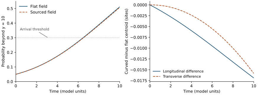
The arrival time is the first crossing of Pdet=0.30 on the tested interval. A second readout is the crossing of ⟨Y⟩=9, about two sites beyond the initial centroid. Both traces are monotone and bracket their thresholds. This defines an ensemble probability readout, not an absorbing detector or a quantum first-passage distribution. About 4.99% of the initial state is already beyond the detector plane.
Table 6. Arrival readouts from the saved time grid, with spacing 0.25. The flat centroid travels 2.60004 sites. At T=10, the curved-minus-flat transverse centroid shift is −0.015856 sites. Times and lengths are in the model’s lattice units.
Readout
Flat
Curved
Curved minus flat
Centroid crossing time
7.690306
7.739277
+0.048972
Detector threshold time
6.477716
6.521907
+0.044191
Detector probability at T=10
0.511272
0.506917
−0.004355
Independent matrix assembly and a short-step exponential series reproduce all 41 saved states in each flight to less than 1.5×10⁻¹⁵ in vector norm. Solving for crossings within the time intervals, instead of linearly interpolating the saved readouts, gives delays 0.048974 and 0.044178. The detector-delay change is about 1.3×10⁻⁵, much smaller than the measured effect. These comparisons validate the numerical evolution and readout; they do not bound lattice or physical-model errors.
Figure 3. The massless packet crosses a specified probability threshold later in the sourced field. Left: detector probability, including its nonzero initial tail. Right: centroid retardation and the transverse curved-minus-flat displacement. Lines join the saved states; no coefficients or trajectories are fitted.
A control experiment checks that the readouts measure motion and not merely phase changes. Removing offsite hopping freezes both positions and detector probability, while retaining the onsite Wilson terms. The massive packet’s lattice momentum still changes by −0.001760 over t=0.6, because spatially varying phases can change momentum without transporting probability. This control distinguishes motion from phase evolution.
The positive delay and inward displacement are substantial improvements over the earlier 0.1257-site flight. They are gravity-like responses to supplied static fields. Establishing a Shapiro prediction or a light-bending angle requires controlled paths, endpoints and propagation limits, and ultimately an appropriate photon model [7]. The next section controls the common readout and finite-time errors for a smooth benchmark. Completing the actual source stress, curved-space propagation limit and gravitational dynamics remains necessary; this arrival experiment does not supply those ingredients.
7 Recovering a supplied geometry with controlled errors
7.1 Separating four sources of error
The preceding experiment shows a delay, but a good-looking ratio alone does not tell us how accurately a packet reads the local geometry. A packet occupies many sites, the field varies across it, the lattice changes its dispersion, and the box has boundaries. Each of these can bias a readout. The controlled-scaling calculation separates these effects by varying one scale at a time and bounding the error each one can cause. Its question is deliberately narrower than deriving gravity: given a smooth static geometry, do clocks and moving probes recover it within an explicit error allowance?
The physical speed parameter is held at c=0.5, the Wilson coefficient at rW=0.5, and the massive and massless probe parameters at M=2 and M=0. Restoring the lattice spacing a in Eq. (37) gives
Thus the hopping coefficient is Ja=c/a: halving the spacing doubles the hopping, so the physical speed stays the same. This change converts the same physical derivative to a different grid; it is not a fit to the measured motion. It also is not a derivation of scale dependence from a microscopic qutrit network. The probes here are the separate Dirac sector of the paper.
To have a known answer to compare with, we supply a simple smooth field rather than the trapped source of the previous section. A smooth Plummer potential supplies the benchmark [11], a softened version of a point-mass potential:
The source is centred at −Rex, while the probes start near the origin. Increasing R makes the field vary more slowly across a fixed packet, with ϕ(0)=−0.01 unchanged. The potential has a positive smooth Poisson density, ∇2ϕ=3As2/(r2+s2)5/2, where r=∣x+Rex∣. This is an analytic reference source, not the trapped matter state of Section 6. In particular, its relation χ=−ϕ is supplied.
The packets are prepared as follows. The physical momentum envelope is exp[−σ2∣k−k0∣2], followed by projection onto the nonnegative lattice band. The massive packet has k0=0; the massless packet has k0=ey. Its directional zero-mode prescription is retained. Nine cases vary one scale at a time about a=0.5, R=64, σ=2, and box half-width B=10: spacings 1,0.5,0.25, field scales 16,32,64, widths 1.5,2,2.5, and half-widths 8,10,12. They are not a full Cartesian sweep. The even grids have coordinates [−B,B−a]3. Their slight asymmetry is retained in every bound.
7.2 What the clocks and forces establish
Write q=ϕ−χ, N0=eϕ(0) and F0=eq(0). Thus N0 is the clock-rate factor and F0 the light-speed factor at the starting point. The clock measures its initial phase-rate ratio Rc; the massless packet measures its initial velocity ratio Rv. With the flat clock’s Wilson fraction w=fW, the exact uniform-field inverse suggests
N=1−wRc−wRv,ϕ=lnN,q=lnRv,γ=ϕq−1.(45)
These formulas turn the two measured ratios into estimates of the local fields, using the fact that the clock rate mixes rest and Wilson contributions in the known proportion w. Unlike the earlier logarithmic subtraction, this inverse does not linearize the field strength. The measurements and flat preparation determine it; the known background enters only the error certificate and the independent comparison. In an inhomogeneous field it is an estimator, with an error that must be bounded.
Appendix H obtains those bounds from the actual site and bond kernels. It also constructs a second estimator, using the massive and massless momentum rates to infer gϕ=∂xϕ(0) and gq=∂xq(0). The reference values are γ=1 and gq/gϕ=2. Both are consequences of the supplied field, not predictions of a gravitational theory.
Table 7. Analytical readout enclosures for the same packets at a=0.5, B=10 and σ=2. The supplied targets are γ=1 and gradient ratio two. The last column retains the signed quadratic contribution and bounds the cubic remainder. Endpoints are printed outwards; floating-point evaluation of the underlying bounds is not interval-certified.
R
Clock–speed γ
Force ratio: second order
Force ratio: signed quadratic
16
[0.59475,1.50697]
Unresolved
Unresolved
32
[0.95572,1.04503]
[1.22430,3.28408]
[1.63018,2.45500]
64
[0.99116,1.00882]
[1.65272,2.42217]
[1.93990,2.06187]
At R=64, the measured values are γ=0.9999698 and gq/gϕ=1.9999348. Table 7 gives the information that those close central values alone cannot provide: deterministic enclosures for the possible readout error. An enclosure is an interval that is guaranteed, by the inequalities, to contain the true value of the readout target. These are analytical inequalities evaluated in floating point, not confidence intervals or outward-rounded machine proofs. If a denominator’s interval reaches zero, the ratio is reported as unresolved.
The force certificate improves substantially when the quadratic field contribution is summed with its sign before the remaining error is bounded. Opposite parts of this packet almost cancel that contribution, so bounding each part’s absolute value separately greatly overestimates the error. The sharper calculation keeps the small residual, including all boundary terms, and bounds the cubic remainder. At R=64 it narrows the enclosure by a factor 6.31 without changing the estimator or any coefficient. It does not require an exactly symmetric box, an exact parity theorem for the state, or a claim that the derivative bound is optimal.
The original compact source remains a useful countercheck. Applying the new inverse to its unchanged L=21, width-two data gives γ=0.96708, but the enclosure is [−0.2956,4.6250]. Its gradient-ratio estimate is 1.93147, while the ratio enclosure is unresolved. The older value 1.9232 belongs to the different first-order inversion and remains in Table 5. The smoother benchmark therefore demonstrates how to obtain control; it does not retroactively certify the earlier source.
7.3 Controlling complete propagation
Initial rates and complete flights answer different questions: the first asks how a probe starts to respond, the second whether its whole motion stays close to a simple description. Five flat and curved flights were computed to physical time T=4: the three spacings at B=10, and the two additional box sizes at a=0.5. They use the full Hermitian Hamiltonians, not the linear response used to motivate a readout.
For the massless packet a simple reference is the locally uniform periodic lattice law, which replaces the varying field by its value at the starting point:
Hloc=F0Ha,per.(46)
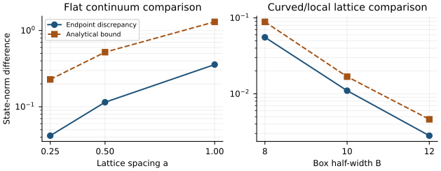
Duhamel’s identity bounds the state difference by integrating the action of the actual Hamiltonian difference on the reference state. In plain terms, the two evolutions can drift apart only as fast as the difference between their Hamiltonians acts on the evolving state. The integral is itself bounded by a vector Taylor remainder; it is not inferred from convergence of a quadrature grid. At a=0.5, B=12, the observed state-norm discrepancy is 0.0028066at T=4, while the bound 0.0046117 holds throughout 0≤t≤4. An endpoint observation is not a measured maximum over that window. The bound concerns this prepared packet, not every input state, and a state-norm error is not a percentage error in every observable.
Figure 4. Two independent error controls under the fixed probe prescription. Left: refining the spacing reduces the flat lattice-to-continuum state discrepancy at T=4 on the same periodic physical box. The bound includes the change in positive-band preparation. Right: enlarging the open box reduces the curved-to-locally-uniform lattice discrepancy at a=0.5. Solid curves join endpoint observations; dashed curves join derived bounds. No convergence exponent is fitted.
The continuum comparator on the left of Fig. 4 is the Fourier Dirac operator on the same periodic box. It is not a spatially varying curved-space solver. Combining that comparison with Eq. (46) gives, at a=0.25 and B=10, an observed curved-to-uniform-continuum discrepancy 0.04299, bounded by 0.24680. The bound is useful but does not establish percent-level complete continuum dynamics.
Table 8. Matched-time error accounting. The first three rows sum to the original total. The lower rows show the two symbol terms separately; replacing the combined RMS by their sum gives the slightly looser final bound. These norm bounds are not probabilities.
Contribution at a=0.25, B=10, T=4
State-norm bound
Curved/open to local periodic lattice
0.02238708
Flat preparation mismatch
0.03477305
Combined flat symbol error, at F0T
0.18963684
Total original bound
0.24679697
Separate Wilson symbol term
0.15942268
Separate derivative symbol term
0.03077928
Total using their separate triangle bound
0.24736210
The bound can be split into contributions to find which approximation limits it. Table 8 resolves which error dominates. About 91% of the original bound belongs to the whole flat-comparator contribution: preparation plus the combined lattice symbol error. It cannot all be attributed to the Wilson term. The Wilson contribution is the largest part of the symbol bound, but the separate derivative and Wilson norms do not add exactly to its original root-mean-square value. All flat entries use the matched time F0T=3.920795; the actual flat discrepancy there is 0.04152265, rather than its T=4 value 0.04177491.
7.4 What this adds to the gravity programme
The controlled calculation establishes a practical intermediate result: clocks, velocities and forces can recover a supplied smooth geometry with explicit errors, and a simpler local law approximates a complete flight with a finite-time bound. Agreement is strongest when field variation across the packet and boundary effects are both controlled. Good agreement of an initial ratio alone remains insufficient to establish continuum dynamics.
The next physical test is to apply this separation of scales to the actual matter source, retaining its support stresses and source errors. Recovering χ=−ϕ after supplying it is not a derivation of that relation. Neither the present test nor the earlier arrival experiment supplies gravitational field dynamics, a Maxwell photon sector, or a common microscopic law joining the Dirac and qutrit constructions.
8 A quantum mediator: slowing clocks and entangling probes
8.1 The Hamiltonian and the question it can answer
This section asks whether a quantum system placed between two probes can both slow their clocks in a common way and entangle them. A classical expectation-value field cannot retain all correlations of a quantum environment. To test that distinction in a solvable setting, use five mediator qubits with Pauli operators Xj,Zj and open ends:
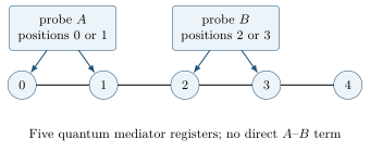
R is the set of positions at which a source acts, s is an overall stiffness and λ is its strength. The mediator has 25=32 states. It is a supplied transverse-Ising spin chain (a standard model of interacting two-level spins in a transverse field), not a qutrit-derived photon or graviton. The positions in this calculation are branch labels; the probes do not hop.
Figure 5. The probe–mediator model. The arrows represent conditional couplings. Both probes interact with the same quantum chain, whose noncommuting dynamics can carry correlations between them.
Let E(R) be the ground energy of Eq. (47). The connected energy shift removes the two individual source energies, leaving only the part that depends on both sources together, which plays the role of an interaction potential:
They show an attractive connected energy contribution that weakens along this finite chain. They do not establish a Newtonian 1/r potential. Open boundaries also mean V depends on both positions, not only their separation.
8.2 Why the clocks approach a common slowing factor
The probe clock is a three-state ring with real symmetric hopping,
The small bond imbalance splits its lowest doublet. There is no complex hopping phase, so this particular clock is not chiral. Couple it to mediator site r through Or=(I−Xr)/2:
HCM=IC⊗HM+HC⊗Or.(51)
In the stiff limit (large s), the mediator remains near its ground state and the leading clock Hamiltonian is ⟨Or⟩HC: every clock is slowed by the same factor ⟨Or⟩, whatever its own frequency. This is the Born–Oppenheimer, or slow-clock/fast-mediator, approximation. Second-order corrections contain HC2 divided by mediator excitation gaps, so they depend on the clock’s own scale and decrease as 1/s.
We compare the lowest-doublet splitting with and without a source at site zero. Three clocks are used, with J=0.5,1,1.5. These are rescaled versions of one clock Hamiltonian, not three unrelated species of physical matter.
Table 9. Clock splitting with the source divided by the splitting without it. Values below one mean slower oscillation in the chosen coordinate time. Agreement improves as the mediator becomes stiff, but finite-s clock dependence remains.
Stiffness; clock position
J=0.5
J=1
J=1.5
s=1, r=1
0.759491
0.780568
0.804338
s=64, r=1
0.742797
0.743025
0.743255
s=64, r=2
0.897287
0.897426
0.897564
s=64, r=3
0.959192
0.959257
0.959321
At r=1, the spread between the three ratios divided by the slowing of the J=1 clock decreases from about 20.4% to 0.178%. The stiff-limit ground-state expectation predicts 0.742570, close to but distinct from the finite-s mean 0.743026. This mechanism explains the observed approach to a common rate. It does not establish universal gravitational coupling across different kinds of clocks, particles or binding energies.
8.3 Entanglement through the mediator
Now give each of two probes two possible positions: A at 0 or 1, and B at 2 or 3. Their joint position space has four states. For each branch (a,b) the mediator evolves under Eq. (47) with those two sources. The total Hilbert space has dimension 4×32=128.
There is no operator acting directly on both probes in the declared Hamiltonian:
HABM=IAB⊗HM(∅)+VAM+VBM.(52)
In this model [VAM,VBM]=0, but each coupling fails to commute with part of the mediator dynamics. The absence of a direct term follows from Eq. (52), not from the commutator alone; two commuting operators can still include a direct interaction.
Each probe starts in an equal superposition of its two positions, so the four branches interfere. The probes begin in ∣+⟩A∣+⟩B. The mediator begins in the ground state of the Hamiltonian averaged over their four branches, giving an initially factorized state. We then evolve the full Hamiltonian, retaining mediator recoil and probe–mediator entanglement. A convenient fixed readout time is
t∗=∣E02+E13−E03−E12∣π,(53)
where the Eab are the four branch ground energies at the chosen stiffness. This adiabatic phase estimate sets a time; it does not replace the full evolution. Because the chain is open, one must use these four energies rather than a formula involving only three separation-dependent potentials.
Table 10. Entanglement after tracing out the quantum mediator. Concurrence ranges from zero to one; two-qubit negativity has maximum 1/2. The weaker source produces less residual entanglement with the mediator and a cleaner entangled probe pair. Values are reproduced by an independent spectral evolution.
Source strength
t∗
TrρAB2
Concurrence
Negativity
λ=2, s=16
1.74398
0.830523
0.819717
0.409336
λ=0.5, s=16
12.69075
0.975984
0.975805
0.487886
Concurrence and negativity are standard two-qubit diagnostics [12, 13]; Appendix C defines them. Both are zero for unentangled states, and larger values mean more entanglement. The purity TrρAB2 equals one when the probe pair is not entangled with the mediator. A control that replaces the mediator operators by fixed expectations leaves a sum of single-probe Hamiltonians. It cannot entangle this initially product pair. That establishes a difference between the full quantum chain and this particular mean-field approximation.
The experiment is inspired by proposals to witness nonclassical gravity through mediated entanglement [14, 15]. Here the mediator’s quantum nature is already supplied. To turn the calculation into a gravitational claim, one would need to derive its coupling to energy, exclude competing interactions, recover the appropriate spatial force law, and establish the locality assumptions of the witness. None follows from observing entanglement in an Ising chain.
9 Entanglement as a test of a graph geometry
9.1 What a minimal-cut law would mean
The final construction concerns a state rather than an evolving Hamiltonian. The idea, borrowed from holography, is that entanglement between regions might itself define distances: strongly entangled regions count as “close”. A tensor with eight quantum legs is placed at each node of a small graph, and internal legs are contracted. The remaining legs define a boundary quantum state. One can then compare a region’s entropy (a measure of how entangled it is with the rest) with the smallest number of graph bonds that separate it from the rest, the minimal cut.
The motivation comes from the Ryu–Takayanagi relation in holography [16] and finite tensor-network models of it [17, 18]. In the present setting a cut through b maximally entangled bonds of local dimension p bounds the entropy by blogp. Equality is a property to test, not an assumption that every tensor network satisfies. A successful graph-cut rule is not the same as deriving a spacetime metric or the coefficient 1/(4G) in gravitational entropy.
We use stabilizer states because their entropies can be calculated by exact finite-field linear algebra [19, 20]. A stabilizer state is specified by a list of commuting Pauli-type operators that leave it unchanged; this list can be written as a matrix of integers modulo p. With entropy measured in units of logp, a pure n-register stabilizer described by G=[X∣Z] has
S(A)=rankFpG∣AX∪AZ−∣A∣.(54)
The rank is over Fp, not over the real numbers. Appendix D explains the formula and gives both tensors explicitly. A bit is the p=2 unit; a trit is the p=3 unit. We compare normalized ranks and deficits, not raw bit and trit quantities as though they were equal.
9.2 The qutrit improves the cut count, but its exceptional cuts are deep
An ideal tensor for this purpose would be maximally entangled across every way of splitting its legs into two halves. The selected eight-qubit tensor has maximal entropy on 56 of its 70 four-versus-four cuts. Its fourteen exceptional cuts have entropy two bits rather than four. The eight-qutrit graph tensor has maximal entropy on 66 of 70 cuts, but its four exceptional cuts also have entropy two, now measured in trits. The initial draft incorrectly assigned them three trits.
This correction can be seen without a large computation. Across one exceptional cut the graph’s 4×4 cross-adjacency matrix has rank two over F3. A direct Schmidt decomposition gives nine equal squared Schmidt coefficients 1/9, hence entropy log39=2. There would need to be 27 coefficients 1/27 to obtain three trits.
The exceptional qutrit subsets, with legs numbered 0 to 7, are
{0,2,4,6},{1,3,5,7},{0,3,4,7},{1,2,5,6}.(55)
They form two complementary pairs. Every one-, two- and three-leg reduction is maximally mixed, and all eight cyclic four-leg intervals are maximal. This is a three-uniform, block-perfect tensor, not an absolutely maximally entangled (AME) tensor. (Three-uniform means every set of up to three legs is maximally entangled with the rest; AME would require the same for every set of up to four.)
These entropy profiles should not be presented as newly established general coding bounds. The sharp eight-qubit count of 56 is due to Zhang et al. [21], rather than a direct statement of the shadow-enumerator reference. The ternary profile (66,0,4)—66 cuts of rank four, none of rank three and four of rank two—also occurs in the classified stabilizer family and is discussed by Dahbi [22], using the code classifications of Danielsen [23]. Our test concerns the displayed tensor, its ordering and its small contracted patch. We do not claim a new AME nonexistence theorem or a necessary local dimension of seven. General entanglement constraints require their own hypotheses [24, 25].
Here AB denotes the union. The monogamy-of-mutual-information (MMI) inequality is I3≤0. Informally, it says that the information region A shares with B plus the information it shares with C cannot exceed what it shares with B and C taken together. It is a necessary entropy property of states described by the classical holographic area formula, but is not obeyed by all quantum states [26]. Satisfying it alone does not establish a holographic dual or all higher entropy inequalities [27].
The qutrit tensor passes despite its two-trit deficits. The reason is where those deficits occur. For a pure eight-party state, introduce the complement D and rewrite
I3=S(A)+S(B)+S(C)+S(D)−S(AB)−S(AC)−S(AD).(57)
This expression is symmetric under permutation of the four regions. There are only five possible sorted size patterns with all four nonempty. The complete argument appears in Appendix D.2. For example, in the (2,2,2,2) case the positive terms total eight. The three distinct balanced cuts can include at most two of the exceptional complementary pairs, so their entropies sum to at least 2+2+4=8. Thus I3≤0.
Exact enumeration confirms zero violations among all 7,770 unordered disjoint triples on the qutrit cell. The chosen qubit cell has 28 violations, with maximum I3=2 bits. The conclusion survives the correction to the exceptional entropies, but the argument must use their incidence as well as their size.
9.4 A nine-cell patch
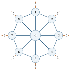
A single tensor cannot show geometry, so we next glue nine of them together. The patch has one central tensor and eight outer tensors arranged in a ring. Each outer tensor connects once to the centre and once to each neighbour. Sixteen internal bonds leave forty boundary legs, five per outer tensor. This is the incidence pattern of a small {8,3} tiling patch: octagons with three meeting at a vertex. It is not an identification of hyperbolic geometry with the earlier octahedral face graph.
Figure 6. The tensor incidence graph, drawn schematically. Blue edges are the sixteen internal contractions. Each outward orange segment represents a bundle of five boundary legs. Edge lengths in this drawing carry no physical meaning.
Table 11. Exact finite-field results. A tile-aligned boundary region contains either all five legs of an outer tensor or none. These tests do not enumerate every subset or every triple on forty boundary legs.
Test
Chosen qubit tensor
Chosen qutrit tensor
Maximal four-leg cuts on one cell
56/70
66/70
Entropy on each exceptional cut
2 bits
2 trits
Single-cell MMI violations
28/7770
0/7770
Connected boundary intervals matching mincut
1560/1560
1560/1560
Tile-aligned subsets matching mincut
240/254
250/254
Tile-aligned ordered MMI violations
168/46620
0/46620
Entropy deficit on exceptional tile subsets
2 bits
2 trits
An independent construction by sequential Bell projections reproduces Table 11, including the corrected two-trit deficits. The source contracts with a charge-conjugated maximally entangled bond; Appendix D states that convention explicitly. A check with ordinary Bell bonds gives the same listed counts on this patch. This finite comparison does not establish bond-convention independence for arbitrary networks.
The result is useful precisely because connected intervals alone fail to distinguish the two tensors: both pass all 1,560 such tests. Disconnected regions reveal their difference. Even the qutrit tensor retains four tile-aligned failures of the minimal-cut equality. No Hamiltonian has yet been supplied that selects this boundary state, and no calculation couples its entropies to the clocks or mediator of the earlier sections.
10 What has been established and what would connect it
This section summarizes what the separate calculations show and what is still needed to join them. The finite calculations identify three requirements for further work. First, a microscopic clock must preserve its full coherent evolution, including spectator amplitudes and finite-gap shifts. The pairing algebra provides a compact way to do that; a large transfer probability at one time is not a substitute for controlling those phases.
Second, a geometry readout needs an error budget before it can test a common dynamical origin. The four-component model uses one kinetic regulator for its source and probes and measures a delayed multi-site arrival. The subsequent smooth-field benchmark adds a controlled separation of scales, finite-strength clock inversion, signed force bounds and a finite-time state comparison. These establish useful recovery of a supplied geometry. They do not certify the original compact source: its force-ratio interval remains unresolved, and the reference source balance is calibrated. The next step is controlled physical-scale refinement of that actual source, including support stresses and source errors. The full stress tensor, spatial Einstein equations, microscopic origin of the field functional and radiative dynamics remain further requirements.
Third, an entanglement geometry needs more than agreement on connected intervals. The qutrit tensor improves the tested disconnected-region behaviour, while its remaining deficits expose the limits of the graph-cut picture. A dynamical extension should ask whether correlations and propagation infer the same changing geometry under one fixed law. Assigning a distance to entropy by definition would not provide that independent agreement.
The defensible result is a set of corrected, reproducible benchmarks and obstructions, now including explicit error bounds for a common probe readout. The transport, mediator and tensor calculations are worthwhile finite-model results. Their combination remains a research programme rather than a derivation of gravity.
Reproducibility and assistance
The supporting code and evidence are archived on Zenodo as version 1.0.0 [28], DOI 10.5281/zenodo.23987418. The archive contains the original hash-pinned scripts, retained review records, replay tools and independent editorial checks. Appendix I specifies which results were recalculated and which are inherited. The paper record also provides the matching LaTeX sources. The earlier clock paper has the DOI given in Ref. [1].
AI assistance was used to restructure the manuscript, check algebra and numerical claims, prepare verification code, identify references and produce diagrams. This disclosure does not replace author responsibility for the scientific claims or independent human review.
A Pairing algebra and the clock reduction
A.1 Representation selection and state counts
This appendix supplies the algebra behind Section 2. Schur–Weyl duality separates the action of collective colour rotations from permutations of the physical qutrits [29]. Each symmetry type is labelled by a Young diagram λ, a list of row lengths of boxes; the permutation multiplicity counts how many independent copies of the corresponding colour representation occur. An eight-qutrit Young diagram λ=(3,3,2) has SU(3) labels (λ1−λ2,λ2−λ3)=(0,1), hence antitriplet colour. Its permutation multiplicity is 42. The selected physical space has dimension 3×42=126.
The class sum Σ8=∑i<jSij commutes with all permutations, so it has a single eigenvalue on each symmetry type. It has eigenvalue
cλ=21i∑λi(λi−2i+1).(58)
For λ=(3,3,2),(4,2,2),(4,3,1) these values are 0,2,4. Thus Hsel=(Δ8/2)Σ8 gives gaps 0,Δ8,2Δ8. In the total-fundamental sector of all ten qutrits, the 210-dimensional permutation multiplicity branches as
The overall triplet colour is a spectator factor and need not be repeated in the multiplicity simulation. “Unprojected 210-state” means that all three S8 sectors in Eq. (59) are retained. The full ten-qutrit Hilbert space is much larger.
There is another 210-state calculation in the original clock work: 42 internal multiplicity states times a five-dimensional fixed-weight colour space. That space belongs to the cluster-projected model and is not the 210-dimensional finite-gap multiplicity above. Equal matrix dimensions must not obscure the different projections.
A.2 The two-dimensional pairing space
For fixed total colour, the pair states of Eq. (4) have Gram matrix (the matrix of their mutual overlaps)
Gpair=(11/31/31).(60)
Taking the first orthonormal basis vector along uAB and the second along the orthogonal component of uBC gives
Changing the sign of the second basis vector changes both off-diagonal signs, with no physical effect. These matrices make the reflection identities and failure of the permutation braid relation explicit.
Let T have columns given by the two pair states, for all three total colours. The active projector is P=T(T†T)−1T†. Direct substitution for v=∣0,0ˉ,2⟩ and w=∣2,1ˉ,1⟩ gives
These numbers give the bounds of Eq. (6). Cauchy–Schwarz bounds the active transition amplitude by 3/8. In the contraction algebra the colour action on the combined spectator space is a scalar, so its contribution is bounded by 1/8, even when an internal clock transition is included. The triangle inequality gives Eq. (6). The full contraction-class bound is tight if arbitrary active unitaries and an independently phased spectator scalar are allowed; a particular calibrated Hamiltonian need not attain it.
HI is the seventeen-parameter internal law, Oj are the six internal pair-exchange correction operators, and the coefficients are the fixed tables in the preserved clock script. The numerical benchmark here retains those tables without further fitting. They are necessary supplied inputs; Eqs. (61)–(67) alone do not determine them. The earlier clock paper and the source package provide the construction and preparation details [1].
For a block decomposition H=(AB†BD), with A acting on the selected low-energy states and D on the excited ones, eliminating the excited block at energy z gives the exact energy-dependent operator
Heff(z)=A+B(z−D)−1B†.(68)
At z=0 and positive D, the return term is −BD−1B†. Calibrating this operator at one energy does not automatically match the entire time evolution. The finite-gap simulation, rather than the zero-energy calibration alone, supplies Table 1.
B Metric and variational details
B.1 Deriving the static vacuum equation
This appendix gives the derivations behind Sections 3 and 4. For hij=e−2ψδij, h=e−3ψ and hij=e2ψδij. Therefore
Dh2N=h1∂i(hhij∂jN)=e2ψ(ΔN−∇ψ⋅∇N).(69)
With N=eϕ, this becomes eϕ+2ψ[Δϕ+∣∇ϕ∣2−∇ψ⋅∇ϕ]. Multiplication by N yields R00 and establishes Eq. (25).
For the flat-spatial candidate N=(1+M/r)−1, the radial flat Laplacian is
ΔN=r(M+r)32M2=0.(70)
For N=1−M/r it vanishes outside the origin, but a spatial component is Rrr=−N−1N′′=2M/(r3N), which does not vanish. This explicitly demonstrates why a lapse-only solution of R00=0 is insufficient.
For completeness, put u=logn and take radial N,u. The independent radial and tangential spatial equations are
The second expression is the component along a unit tangential direction in the flat Cartesian reference frame. Substituting Eq. (27) makes both expressions and R00 zero. These are exact symbolic checks in the editorial audit.
B.2 The source expansion
We now show why freezing the matter state and letting it respond give different nonlinear coefficients in Table 2. Let G=L−1 on the Dirichlet box. Expanding ϕ=κϕ1+κ2ϕ2+⋯ in Eq. (19) gives
ϕ1=−Gs0,ϕ2=−GDs0[ϕ1].(73)
For a frozen state, Ds0 is the Hessian of its matter energy with respect to the field. For a variable state it also includes the state’s linear response. If the chosen eigenvalue is nondegenerate within the selected parity sector,
δ∣χ⟩=n=0∑∣n⟩E0−En⟨n∣δH∣χ⟩,(74)
with phase fixed by ⟨χ∣δχ⟩=0. All other states in that parity sector enter the sum, including negative-energy states. This is why the variable-state coefficient is not determined by the explicit exponential weights alone.
The quoted coefficient estimates use κ=±10−4, combined in the standard symmetric finite-difference formulas:
ϕ1≃2δϕ(δ)−ϕ(−δ),ϕ2≃2δ2ϕ(δ)+ϕ(−δ).(75)
Both have truncation and floating-point error. Their agreement between implementations is a numerical check, not an exact rational certificate. In particular, a very small stationary residual establishes that the chosen finite equations have been solved accurately; it does not establish that those equations represent gravity.
C Quantum mediator observables
This appendix explains the residual clock dependence in Table 9 and defines the entanglement measures of Table 10. For mediator ground state ∣0⟩ and excited states ∣n⟩ with energies En, a clock eigenvalue ϵ in Eq. (51) shifts the mediator ground energy by
Since the mediator gaps grow with s, the quadratic contribution is of order ϵ2/s. The leading clock splitting is proportional to ⟨Or⟩, while the next term depends on the sum as well as the difference of the two clock levels. This gives a concrete mechanism for the residual scale dependence in Table 9.
To measure probe entanglement we must first discard (trace out) the mediator. Write the evolved probe–mediator state as ∑a,b∣ab⟩∣vab(t)⟩. Tracing out the mediator gives
(ρAB)ab,a′b′=⟨va′b′(t)∣vab(t)⟩.(77)
This retains the overlaps between different mediator branches; replacing them by arbitrary independent phases would change the purity and entanglement. The independent calculation obtains each vab by spectral decomposition of its 32×32 branch Hamiltonian. The source instead exponentiates the full 128×128 operator. They reproduce Table 10.
Define ρ~=(σy⊗σy)ρ∗(σy⊗σy). If r1≥r2≥r3≥r4 are the square roots of the eigenvalues of ρρ~, concurrence is
C=max(0,r1−r2−r3−r4).(78)
Here ρ∗ is the complex conjugate. Negativity is N=(∥ρTB∥1−1)/2, where ρTB is the partial transpose (transposing only probe B’s indices) and ∥⋅∥1 is the sum of absolute eigenvalues; it is equal to minus the sum of negative eigenvalues of the partial transpose. Both are positive in the two full quantum runs. The fixed-expectation control factorizes as UA⊗UB and hence has zero entanglement exactly in arithmetic without roundoff.
The general inference from mediator-generated entanglement to a nonclassical mediator requires specified locality and admissible classical operations [14, 15]. Our factorized mean-field control tests only one classical approximation. It does not classify every classical or hybrid gravitational model.
D Tensor specification and exact entropy checks
D.1 The two cell states
This appendix specifies both tensors completely and proves the entropy statements of Section 9. The binary cell is the CSS stabilizer (a stabilizer built separately from X-type and Z-type checks) generated by G2=diag(H,H), where
For this graph-type state the entropy has a particularly simple form. The cut entropy is the rank of (M3)A,Aˉ, the block of M3 connecting legs in A to legs outside it. Across A={0,2,4,6} this matrix is
0102222100002122(mod3).(82)
The first and third rows coincide; the fourth is twice the second modulo three. Two rows are independent, so the entropy is exactly two trits. The explicit-state Schmidt calculation confirms the rank result independently.
For a general pure stabilizer with n independent generators, the subgroup supported entirely in A has dimension n−rankG∣Aˉ. Its reduced state is flat on a space of dimension p∣A∣−n+rankG∣Aˉ. Taking its logarithm gives S(A)=∣A∣−n+rankG∣Aˉ. Purity, S(A)=S(Aˉ), gives Eq. (54). This derivation explains both the finite field and the subtraction of ∣A∣ in that formula.
D.2 The full single-cell MMI proof
The proof checks every way of splitting the eight legs into regions, using the symmetry of Eq. (57) to reduce the work to five cases. If the complement D is empty, purity makes I3=0. Otherwise, all four regions are nonempty and Eq. (57) is symmetric under their permutations. The five sorted partitions of eight suffice:
Region sizes
Reason
Upper bound on I3
(1,1,1,5)
6−(2+2+2)
0
(1,1,2,4)
4+S4−(2+3+3), S4≤4
0
(1,1,3,3)
8−(2+S4+S4′); at most one deficit
0
(1,2,2,3)
8−(3+3+S4), S4≥2
0
(2,2,2,2)
8−(S4+S4′+S4′′); at most two deficits
0
For (1,1,3,3), the two balanced unions have an intersection of size one. Distinct exceptional sets in Eq. (55) intersect in either zero or two elements. Both unions therefore cannot be exceptional. For (2,2,2,2), the three unions are distinct and none is the complement of another: all contain the same nonempty region. The exceptional sets supply only two complementary pairs, so at most two of the unions are exceptional. These incidence facts complete the proof. A bound using only S4≥2 would not suffice in these two cases.
D.3 Contraction convention and patch coverage
This subsection fixes exactly how the nine tensors are glued, so that the counts in Table 11 can be reproduced. Number the central tensor zero and the outer tensors 1+j, j=0,…,7. Connect central leg j to outer leg zero, and outer leg seven to leg one of the next outer tensor. The remaining legs 2,3,4,5,6 are the boundary of each outer tile.
For ternary registers the source uses the bond bra associated with
∣Φ−⟩=31x=0∑2∣x,−x⟩.(83)
It has stabilizers X⊗X−1 and Z⊗Z. A surviving product stabilizer therefore obeys xa+xb=0 and za−zb=0 on each paired pair of legs. The independent method performs these two commuting measurements bond by bond and then removes the measured legs. It obtains forty independent boundary stabilizers. The same listed counts also hold when the bonds use Φ+=3−1/2∑x∣x,x⟩, checked separately rather than assumed.
The minimal cut is found by enumerating all 29 assignments of tensor nodes to either side. A crossing internal bond costs one, as does a boundary leg whose assigned tensor side disagrees with the chosen boundary region. Entropies are calculated independently by finite-field ranks. There are 40×39=1560 labelled proper connected intervals, including complementary intervals separately. There are 28−2=254 nonempty proper tile-aligned subsets. Their ordered disjoint triples number 46620=6×7770. These conventions explain the counts and prevent a tile-level test being mistaken for an exhaustive forty-leg test.
E The two-potential benchmark in detail
E.1 The actual bond operator and its dispersion
This appendix supplies the details behind Section 5: the exact bond operator, which Einstein equations the two Poisson equations represent, and the controls on the local readouts. For an undirected nearest-neighbour bond, the new source script implements
At a bulk site six bonds contribute a total onsite term 3Jσz. The two directions along axis i contribute −Jcoskiσz+(J/2)coskiσx. Adding them gives Eq. (35). The off-diagonal term is even in momentum and nonzero at k=0; setting M=0 therefore does not produce a massless Dirac point. Completing the square gives Eq. (36), a bound throughout the bulk Brillouin zone (the full range of lattice momenta), not merely a finite-grid observation.
The sparse independent construction uses the graph adjacency matrix A and degree matrix D. At flat fields the bond sum is
Hbond=2J(D−A)⊗σz+4JA⊗σx.(85)
This reproduces the source matrix and its selected energies. A separate periodic real-space construction reproduces the Bloch operator. The source derivatives were also checked by directional finite differences using a complex matter state, without relying on the source’s real-eigenvector implementation.
E.2 Which Einstein equations are represented
For h00=−2ϕ, hij=2χδij and no time dependence, linearizing the Ricci tensor gives
Equations (31) match the first and last of these after the identifications stated in the main text. Their derivation is also consistent with restricting the static Einstein–Hilbert action before variation: for the spatial metric e2χδij, its curvature is e−2χ[−4Δχ−2(∇χ)2]. Integration by parts yields the quadratic static action density proportional to 2∇ϕ⋅∇χ+(∇χ)2, with the opposite sign in the energy functional. Boundary conditions must be specified in this step [3].
A restricted variation, one that allows only the two scalar fields to vary, cannot supply every component equation. For example, ϕ+χ=x2−y2 is harmonic and satisfies the spatial vacuum trace, but Gxx=−2 and Gyy=2. This local counterexample is enough to show why a Poisson trace test alone is insufficient. It is not a proposed isolated solution with the protocol’s boundary conditions. A finite-box scalar source also does not specify the complete anisotropic matter stress needed on the right-hand side of Eq. (88).
The next calculation asks whether the field energy is positive in every direction, a first test of stability. For a normalized Laplacian eigenvector with eigenvalue ℓ>0, write the field perturbations as (a,b) in that mode. The field part of the Hessian of Eq. (30) is
κℓ(0−1−1−1),λ±=2κℓ(−1±5).(89)
One eigenvalue is negative and the other positive. This is an unrestricted field Hessian, not a physical-mode stability theorem: constraints and matter variations have not been eliminated. It explains why the single positive scaling curvature reported by the protocol cannot be called positive-definite ADM stability.
E.3 Controls that distinguish a readout from motion
Deleting the intersite blocks while retaining the onsite diagonal leaves the protocol’s clock-versus-matter readout unchanged. Yet the resulting Hamiltonian commutes with position and cannot transport a packet. This provides a direct control on what that comparison measures.
For the original small hopping J=10−5, an upper-component state localized at the specified r=2 site has initial ∣d2⟨X⟩/dt2∣ of order 10−13 from the double commutator. The onsite-energy proxy has magnitude 1.273985×10⁻³. The localized state is not a smooth continuum packet, so this example is not a continuum force measurement. It demonstrates that the proxy is not an operator identity for the stated lattice dynamics.
Likewise, a real equal-amplitude internal state has bond current −2Im(ψu†Huvψv)=0 for the real bonds used here. Reading their magnitude cannot establish directed propagation. A useful replacement test would evolve a packet with a verified dispersion and compare arrival times or integrated trajectories with clock readings, keeping the couplings fixed.
F Dirac packet law and readout diagnostics
F.1 Bond Hamiltonian and source identities
This appendix gives the explicit Dirac lattice law of Section 6 and documents the earlier short-flight readout whose problems motivated the newer experiments. For a bond from site u to its neighbour v=u+d^, the new Hermitian operator is
The first term is the antisymmetric lattice derivative. The second is the Wilson term; its endpoint diagonals belong to the bond and must be retained when differentiating its field weight. With Vu=(σ0/2)∣xu−xc∣2 and Wu=−Vwelle−∣xu−xc∣2/2, the full law is
Every term acquires the same factor under a uniform lapse shift, proving the first identity in Eq. (39). Under a uniform spatial shift the trap receives a factor e2ϵ and each entire bond a factor e−ϵ. This proves the second identity, including the Wilson endpoint terms. Combining the shifts gives the third. All are derivatives at a fixed state; the Hellmann–Feynman theorem (the derivative of an eigenvalue equals the expectation of the derivative of the Hamiltonian) permits the corresponding eigenvalue derivative on a differentiable eigenbranch.
Fourier transformation gives Eq. (37). Squaring it removes the cross terms because {αi,αj}=2δijI and {αi,β}=0, proving the dispersion relation. For M=0 and rW>0, vanishing energy requires both every sine to vanish and every nonnegative 1−coskd to vanish. Thus only the origin survives: the Wilson term removes the unwanted massless modes. For rW=0 the latter requirement disappears. The eight spatial corners are inequivalent zeros in the Brillouin torus. This species count concerns the translation-invariant bulk, not an exact zero eigenvalue of a finite open box.
For an αy=+1 spinor z with z†z=1, the pure Dirac hopping block is Huv=−iJαy/2. The outgoing bond probability current for ψv=eikyz is
ju→v=−2Im[z†Huveikyz]=Jcosky.(92)
This distinguishes the current from the sine appearing in the energy operator. The Wilson current expectation vanishes for that spinor because ⟨β⟩=0; this does not make it a Wilson energy eigenvector.
F.2 The earlier short-flight readout
The following formulas describe the earlier rW=0 probe experiment, retained to explain the corrections that motivated the common-regulator study. Let Tx=∑u:u+x^exists∣u⟩⟨u+x^∣⊗I4. Define the finite-lattice operators
These are the lattice versions of momentum and of the identity. On a periodic plane wave these are sinkx and coskx, rather than the unbounded canonical momentum and the identity. Their expectations therefore matter for broad-momentum packets.
The clock preparation superposes the two β sectors. Its coherence is measured with O−=(σx−iσy)⊗I2, summed over sites. Linear fits to arg⟨O−(t)⟩ define ωcurved and ωflat. The reported clock estimator and its symmetric difference are
This is an operational phase-rate definition. With finite hopping, finite width and a finite fit interval, it is not identically the field at the packet centre or an exact convolution with its initial density.
Subtract curved and flat momentum histories. If δP˙m denotes the fitted early rate for the massive packet, the comparison uses
The first expression approximates a slowly varying force by a packet energy times a gradient. The second uses the expected relation between a local speed factor eϕ−χ and a clock factor eϕ. These are model-based estimators, even though their input numbers come from evolution. The exact momentum equation is d⟨Px⟩/dt=i⟨[H,Px]⟩; it generally contains correlations that do not factor into E⟨Cx⟩ times a single gradient. The exact position equation also implies [H,X]=0 for an onsite Hamiltonian, while [H,Px] need not vanish. In the no-hop massive control the final momentum change is about −0.0012023, despite constant position probabilities.
F.3 Testing the proposed overlap correction
The earlier analysis also applied a correction factor to the massless packet’s force, which we test here. The source divides the massless impulse estimator by
fproposed=1−EℓEx(1−⟨Cx⟩ℓ3),(96)
where Ex is its flat x-bond energy and Eℓ its total flat energy. This gives 0.9079799 for the actual prepared packet. No general identity turns a two-step, spin-weighted overlap into a power of the one-step expectation. Both the spinor preparation and open boundaries matter.
An exact diagnostic supplies a linear perturbation of the massless, rW=0 bond weights, fuv=1+ϵ(xu+xv)/2. If H0 is the flat hopping matrix, its derivative is D={X,H0}/2. Thus the exact initial force per unit ϵ and its normalized factor are
Independent finite differences of the weighted Hamiltonian confirm this derivative. The discrepancy of 0.06851 from Eq. (96) shows that the latter is not an exact overlap identity for this state. The actual sourced field is inhomogeneous, so Eq. (97) must not simply replace it as a new fitted correction. A controlled readout would evaluate the appropriate commutators and bound the finite-packet and field-gradient approximations.
Finally, the source’s local massless preparation is (I+H⊥/(2Jsink0y)) applied to a Gaussian spinor, followed by normalization. It is a first-order spinor approximation, not the exact projector (I+H0/E)/2. Fourier decomposition in the stated flat periodic reference gives 3.1054% negative-band weight and 0.8982% in the zero-energy momentum block. These are preparation diagnostics in that reference; open-boundary evolution does not commute exactly with its projectors. They do not contradict the measured trajectories, but exclude a claim that an exactly positive-energy massless state was propagated.
G Exact response identities and the common-regulator readout
G.1 The Wilson boundary term
This appendix derives the exact formulas used to turn probe responses into field estimates in Section 6, and records the checks on the arrival experiment. The flat untrapped probe Hamiltonian separates as H0=Ho+Hb, where Ho=MI⊗β and Hb contains every complete bond in Eq. (90). To test a spatial gradient, set
ϕu=ϵgϕ(xu−xc),χu=ϵgχ(xu−xc).(98)
The quantities gϕ and gχ specify fixed slopes; ϵ is the expansion parameter. With X=X−xcI, direct differentiation at ϵ=0 gives
Here Πx=j projects onto sites in the indicated boundary plane, before the four-component internal factor is included. The correction arises because the bond weight is evaluated at the midpoint, whereas the Wilson bond has diagonal entries at both endpoints. For a linear x gradient, their mismatch cancels at every interior site. Only the two boundary planes remain, with opposite signs. Omitting this term gives a matrix-entry error of 0.0625 at J=rW=0.5. Independent bond-by-bond assembly matches Eq. (100) to floating-point roundoff; finite differences check the full derivative separately. The exact statement is the matrix identity derived above.
For a fixed normalized initial state define
Wo=−i⟨[Do,Px]⟩,Wb=−i⟨[Db,Px]⟩.(101)
These are state-dependent response coefficients: they say how strongly a given packet’s momentum responds to each kind of gradient. Subtract the flat rate and use Ehrenfest’s equation (the rate of change of an expectation value is the expectation of i times the commutator with H) to obtain
This is an exact derivative identity, with the stated remainder for the exponential coupling law. It is not an exact finite-gradient force formula. Subtracting the flat rate is also necessary: boundaries and initial preparation can contribute to the unsubtracted commutator.
For the massless probe Ho=0, so Wo=0. The study applies Eq. (102) to the actual source field by defining
The massless packet has no onsite term, so it measures the bond gradient alone; the massive packet then gives the remaining lapse gradient. Subscripts ℓ and m denote massless and massive packets. The reported two-weight ratio is gb/gϕ. In a weak common linear gradient this recovers (gϕ−gχ)/gϕ. For extended packets in the sourced field, the two states sample different spatial correlations. The measured number 1.9232 is consequently an approximate field diagnostic, not an exact reconstruction of two local metric gradients.
G.2 Clock and velocity normalization
This subsection gives the exact uniform-field version of the clock correction and the correct velocity normalization. The initial register-clock coherence is real and equals one in the stated normalization. Its phase rate can therefore be obtained directly from i⟨[H,O−]⟩. For spatially uniform ϕ,χ, the flat clock frequency splits into rest and Wilson contributions. If fW is the Wilson fraction defined in the main text, the exact ratio is
Rclk=(1−fW)eϕ+fWeϕ−χ.(104)
The longitudinal velocity operator contains bond terms, so for the same initial state in uniform fields Rv=eϕ−χ. The exact uniform inverse, when its logarithm has positive argument, is then
ϕ=ln(1−fWRclk−fWRv).(105)
Expanding this identity to first order gives Eq. (41). Neither uniform formula is asserted to be exact for the inhomogeneous source. As a diagnostic, uniform fields (ϕ,χ)=(0.2,−0.3) on a small box give 0.2 from Eq. (105) and 0.2010312 from the linear logarithmic rule. No replacement correction was fitted to the propagation data.
For any Hermitian H and position operator Y, the velocity is
dtd⟨Y⟩=i⟨[H,Y]⟩=2Im⟨Ψ∣YH∣Ψ⟩.(106)
The producer’s intermediate variables use the last expression without its factor of two. Their ratio, and hence both reported γ diagnostics, is unchanged. The paper uses the normalized equation. For the widest L=21 massless packet, the true flat initial speed is 0.3352293, twice the intermediate value 0.1676147. The separate long-flight centroids come from evolved state vectors and do not use this variable.
G.3 Band content and arrival verification
For each nonzero-energy momentum block, the projector is P+(k)=[I+HD(k)/E(k)]/2. At k=0 in the massless case the implementation uses (I+αy)/2, the directional cone limit. This retains zero-energy norm; it does not remove it. An independent construction by spectral diagonalization reproduces all massive and massless prepared packets within 4.7×10⁻¹⁶ in norm. The high-momentum fraction, defined by maxd∣kd∣>π/2, falls from 0.0449 to 0.00020 as width increases from one to two in the L=21 census. Suppression of this fraction is useful preparation evidence, but central momentum remains fixed and it is not a continuum extrapolation.
The original flight stores 41 vectors over 0≤t≤10. Independent propagation uses a separately assembled sparse Hamiltonian and a 24-term exponential series on steps of 0.25. It reproduces those vectors, including their phases, within 1.5×10⁻¹⁵. Thresholds are checked to lie between the endpoints of monotone traces. Root finding on the independently evolved state within each crossing interval gives
Refined crossing
Flat time
Curved time
Delay
⟨Y⟩=9
7.69030325
7.73927679
0.04897354
Pdet=0.30
6.47788592
6.52206377
0.04417786
The displayed extra digits document numerical comparison, not physical accuracy. These are model-time crossings; no emitter–receiver proper-time comparison, absorption dynamics or continuum error bound is supplied. The no-hop control is checked independently by exact onsite phase evolution, retaining all Wilson diagonals.
H Readout and propagation error bounds
H.1 A finite-strength expansion of the actual bond law
This appendix gives the error calculation underlying Section 7. Its inequalities hold in real arithmetic for normalized states. Their recorded numerical evaluations use double precision. The distinction matters: a mathematical bound and an outward-rounded implementation of that bound are different products.
Here Ou is the onsite mass matrix and Bb is the complete unweighted bond matrix, including both Wilson diagonals. A bond b=(u,v) is not assigned the exponential of the field at its midpoint. That seemingly small replacement would change the quadratic coefficient below.
The strategy is to Taylor-expand each exponential weight around the packet’s starting point and bound everything beyond the first-order term. Let mb=(xu+xv)/2, and let Gϕ,Hϕ bound the gradient norm and Hessian operator norm on the convex box. The symbols Gq,Hq have the same meaning for q. Expanding the site along λxu and the bond along its two endpoints λxu,λxv gives
The gradients gϕ,gq are evaluated at the origin. The factor a2/4 follows from (∣xu∣2+∣xv∣2)/2=∣mb∣2+a2/4. These are finite-strength exponential bounds, not a truncation in the small potential amplitude.
The bounds need the largest gradient and curvature of the field anywhere in the box. For the Plummer field, write D=r2+s2. The gradient magnitude is Ar/D3/2; the two tangential Hessian eigenvalues are A/D3/2 and the radial one is A(s2−2r2)/D5/2. The bounding radial interval is
r−=max(R−B,0),r+=(R+B)2+2B2.(110)
Endpoints and the stationary radii s/2 for the gradient and s3/2 for the negative radial Hessian suffice, with a stationary point used only if it lies inside the interval. The tangential Hessian magnitude decreases with radius. These are analytic suprema on an enclosing radial interval, not derivative maxima sampled at the lattice sites. Here Gq=2Gϕ and Hq=2Hϕ.
H.2 Clock and speed errors before taking a ratio
We next bound the clock and speed readouts. Each is a weighted average of the site and bond factors, so its error follows from the bounds above. For a real normalized clock envelope fu, its unweighted Wilson energy is
Thus ∣Rc−[(1−w)N0+wF0]∣≤Ec and ∣Rv−F0∣≤Ev. The inverse in Eq. (45) consequently obeys
∣N−N0∣≤EN=1−wEc+wEv.(115)
Propagate [N−EN,N+EN] and [Rv−Ev,Rv+Ev] through the logarithms and their ratio. A nonpositive logarithm argument or a denominator interval containing zero leaves the ratio unresolved. No statistical error model is introduced.
H.3 A third-derivative envelope with a proof
The sharper force bound keeps the second-order term exactly, so it requires one further derivative: a bound on the third derivative. For a unit vector u, set z=r⋅u and b=r2/(r2+s2). Direct differentiation gives
D3ϕ[u,u,u]=(r2+s2)5/2Ar(−9z+15bz3).(116)
The expression is zero at r=0 by continuity. Since 0≤b≤1 and ∣z∣≤1, its bracket has absolute value at most nine. To see this, take z≥0 by oddness. When the bracket is negative its magnitude is at most 9z≤9; when positive, 15bz3−9z≤15z3−9z≤6. Hence the valid bound is
The envelope grows until r=s/2 and decreases afterwards, which explains the clipped radius. We require only directional derivatives along the Taylor paths. We do not identify this envelope with an exact tensor norm: at r=s/2, the bracket is −9z+3z3 and its maximum magnitude is six, not nine.
Let Hϕ and Hq be the Hessian matrices at the origin. The quadratic terms in the site and bond expansions are
The endpoint correction in Eq. (119) comes from the Hessian part of the two-endpoint path. The squared-gradient part uses the mean displacement. Neither evaluating everything at the midpoint nor averaging two separate endpoint exponentials gives the same formula.
For the bond, put qˉ(λ)=[q(λxu)+q(λxv)]/2. Differentiating eqˉ three times gives eqˉ[(qˉ′)3+3qˉ′qˉ′′+qˉ′′′]. If μj=(∣xu∣j+∣xv∣j)/2, the estimates μ13≤μ3 and μ1μ2≤μ3 bound all three terms. Taylor’s integral remainder then supplies the factor 1/6. This proves the bond estimate without replacing the actual transport coefficient.
H.4 Signed force moments, with no parity assumption
The force on a packet is a sum of site and bond contributions, each multiplied by its field factor. Set p=Pxψ, where Px is the open-box central-difference momentum. The force kernels, the per-site and per-bond contributions, are
They give −d⟨Px⟩/dt=∑kuNu+∑kbFb exactly. With all sums over the actual finite array, define
Ab=b∑kb,Wo=u∑kuxu,Wb=b∑kbmb,x.(123)
The uniform onsite contribution vanishes because [Mβ,Px]=0. The benchmark’s two gradients are along x, so there are no omitted transverse linear terms. Subtract the flat force and (Rv−1)Ab from the curved force to form f. Then
The earlier bound replaced this by B2=∑∣ku∣Uu(2)+∑∣kb∣Vb(2). Equation (125) is valid even when its first term is large: cancellation improves its numerical value, but is not a premise of the inequality.
Interior kernels for the selected packets are numerically odd under (x,y,z)↦(−x,y,−z). The benchmark Hessian is diagonal, making its relevant quadratic form even. This explains the observed small signed sum, but it is not a general symmetry proof: xy and yz would be odd quadratic terms, the massive spin-up seed is not an eigenstate of the associated spin rotation, and the finite box has an unmatched slice. No such term or slice is set to zero in Eq. (125).
For the two packets, with labels m and ℓ, the estimators and bounds are
The true gradients appear in the certificate, not in the estimators: the estimators use only measured quantities, while the bounds may use the known benchmark field. Ratio intervals are obtained from the full rectangular enclosure of the two gradients, not by linear error propagation. This loses possible error correlations but preserves a valid bound.
H.5 Finite flights and the continuum budget
Finally we bound complete time evolutions rather than initial rates. For two bounded Hermitian Hamiltonians H and H0 acting on the same initial state, Duhamel’s identity gives
∥e−itHψ−e−itH0ψ∥≤∫0t∥(H−H0)e−isH0ψ∥ds.(128)
For K=H−H0, a reference state ψj=e−itjH0ψ, and an interval of width d centred at tj, its contribution is at most
d∥Kψj∥+4d2∥KH0ψj∥+24d3∥K∥∥H02ψ∥.(129)
This follows by expanding the reference vector to first order and bounding its second derivative using unitarity. Summing 64 intervals bounds the integral through T=4. Since its integrand is nonnegative, the same total bounds every shorter time. For the curved/local comparison use H0=F0Ha,per and the full curved open-box operator in K.
The numerical evolution itself uses a truncated exponential series, whose error needs a bound on the size of H. The safe operator bound used for the evolution is
∥H∥≤MNmax+3(c/a)Fmax(1+2rW).(130)
The open Wilson Laplacian is an edge-incidence matrix product D†D with norm at most four in each direction. It is not (I−S)(I−S†) for a truncated shift S, which has a different endpoint diagonal. Thus the bound includes the actual open-edge law. A 26-term exponential series with step size satisfying ∥H∥Δt≤2 gives a total analytical truncation bound below 2.2×10⁻¹⁸ in the recorded flights. Floating-point roundoff is separate; observed norm drift is below 3.6×10⁻¹⁵.
To compare the lattice with the continuum, we bound how far each lattice momentum block differs from its continuum counterpart. For the periodic Fourier continuum comparator Hc(k)=cα⋅k+Mβ, define
The elementary sine and cosine remainders bound ∥Ha−Hc∥ by ba in each momentum block. If ψa and ψc are the separately normalized lattice and continuum band preparations, Duhamel’s identity gives
∥e−itHaψa−e−itHcψc∥≤preparation∥ψa−ψc∥+combined symbol boundtk∑ba(k)2∥ψc(k)∥2.(132)
The Fourier Gaussian tail outside the retained band is bounded separately by monotone sums and Gaussian integrals in the evidence package. The comparator remains periodic on the same physical box; this does not remove finite-volume or spatially varying continuum errors.
For the locally uniform comparator, evaluate Eq. (132) at t=F0T, then add Eq. (128)’s curved/local bound. Writing ρk=∥ψc(k)∥2, the symbol RMS contains
The square root prevents interpreting separate RMS contributions as an additive percentage budget. This is why Table 8 gives both the original combined bound and the slightly looser triangle decomposition, and attributes the 91% share to the whole flat comparison.
I Evidence, corrections and reproducibility
This appendix records which results were recalculated, which were inherited, and how independently each was checked. The source package preserves the original draft, the later two-potential, wavepacket and common-regulator revisions and all five source scripts byte for byte. Their SHA-256 identifiers are:
The first is verify_joint_gdc_qutrit_network.py; its 58-check result and clock numbers are supported by the two preserved prior review/replay records. The full large suite was not rerun for this editorial revision. The small colour contraction algebra, overlap bounds and vacuum equations were checked independently here.
The second is verify_speculative_gravity_completion.py. It was rerun unchanged and passed all 18 of its own checks. That is not a blanket validation of its interpretation. In particular, its vacuum check expands a supplied reciprocal lapse without testing whether it solves R00=0, and its entropy checks count maximal cuts without checking the entropy of each deficient cut. Both omissions allowed errors in the draft to coexist with a passing suite.
Independent checks reconstruct the two-band Hamiltonian, mediator and finite-field matrices without importing their producer. They reproduce the corrected scalar and mediator tables, vacuum equations and deficient-cut Schmidt rank; a separate sequential-projection method reproduces the patch counts. Deliberate faults are detected. Finite-field calculations are exact; floating-point spectral calculations are not interval-certified proofs.
The third script is verify_unified_gravity_protocol.py. Its unchanged replay passes 9/9 checks and reproduces the reported numerical output apart from runtime. A separate 30-check review reconstructs its Hamiltonian and sources, independently solves its Poisson equations, verifies its bulk dispersion and recomputes its final fixed point. It also tests the restrictions explained in Section 5: state-dependent trap calibration, readouts that survive removal of transport, the missing massless branch, the incomplete spatial equations and the difference between a one-direction curvature and physical stability. Three deliberate faults cause three of the 30 review checks to fail. The incoming source’s nine passing rows are retained as evidence of numerical reproduction, not as validation of their broader physical labels.
The fourth script, verify_fixed_law_wavepacket_evolution.py, replays 7/7. A separate 24-check audit reconstructs its Hamiltonians and local derivatives, solves the fields by sparse elimination, and reproduces packet and saved clock vectors with an exponential series. Three deliberate faults fail three rows. The audit diagnoses the regulator change, special-momentum current test, incomplete band projection and unproved overlap correction. Four disclosed configurations test sensitivity without selecting new fitted parameters. They are review diagnostics, not a continuum extrapolation or preregistered research results.
The fifth script, verify_common_regulator_convergence.py, passes seven new checks and three inherited source checks. A separate 23-check audit assembles the matrices independently, verifies the boundary derivative bond by bond, reconstructs preparations by spectral diagonalization, and reproduces all saved long-flight state vectors by short-step series evolution. It also refines both crossing times. Three deliberate faults fail exactly their three intended rows. Original scripts and reported disagreements are preserved. The source’s grid and detector specifications contain transcription errors; the paper uses the replayed values. The review further qualifies continuum claims, retained zero-mode weight, approximate clock correction and the missing factor of two in a velocity variable. The latter cancels in the speed ratio. These computational reviews are not independent human peer review or interval-certified error bounds.
The controlled-scaling package adds nine preselected initial-rate cases, the unchanged compact-source diagnostic and five full flights. Its scaling/legacy suite passes 90/90 checks, propagation 35/35 and a symbolic/sparse audit 13/13. Boundary and velocity faults each give 11/12; a wrong spatial coupling gives 7/12, all with exit status one. An external audit was subsequently supplied. Its signed-quadratic improvement was independently derived and implemented using the frozen force kernels: 40/40 checks pass, while missing-endpoint and reduced-cubic-bound fixtures each give 5/6 and exit one. This verifies the new certificate; it is not a separate reimplementation of the whole Hamiltonian. All 60 original package hashes and all 20 intake hashes are preserved in the accompanying evidence. The stricter parity and derivative statements and the matched-time error accounting are proved in Appendix H.
The original runs retain a real/complex dtype crash, the first underflowed Fourier-tail report, the earlier propagation outputs and the subsequent unused massive-helper correction. The finite-time extension and sharper force certificate are dated additions, not silently incorporated into the original registration. The latter was proposed after the initial results. No trajectory, coefficient or physical parameter was refitted. The present editorial verification checks the new derivations, table extraction and evidence integrity; earlier unmodified results retain their stated verification scope.
The original draft also cited local MMI review paths that are absent at the supplied repository location. Their claimed findings are not treated as independently inspected evidence here. The cell and patch claims instead rest on the preserved producer replay and the new calculations.
The accompanying review records document the corrections, numerical replacements and reference decisions. Original scripts are unchanged; no new fit to masses, mixing angles or evolution outputs was introduced. This is a research preprint; computational checks do not replace independent human review.
References
David Elliman. Qutrit clocks and colour: Pairing algebra and finite-gap transport. Zenodo, 2026. Research preprint, version 2.0. Concept DOI: 10.5281/zenodo.23900249.
H. N. V. Temperley and E. H. Lieb. Relations between the ‘percolation’ and ‘colouring’ problem and other graph-theoretical problems associated with regular planar lattices: some exact results for the ‘percolation’ problem. Proceedings of the Royal Society of London A, 322: 251–280, 1971. doi:10.1098/rspa.1971.0067.
Richard Arnowitt, Stanley Deser, and Charles W. Misner. Republication of: The dynamics of general relativity. General Relativity and Gravitation, 40: 1997–2027, 2008. doi:10.1007/s10714-008-0661-1. Reprint of the chapter in L. Witten (ed.), Gravitation: An Introduction to Current Research, Wiley, 1962, pp. 227–265.
Sergey Bravyi, David P. DiVincenzo, and Daniel Loss. Schrieffer–Wolff transformation for quantum many-body systems. Annals of Physics, 326: 2793–2826, 2011. doi:10.1016/j.aop.2011.06.004.
Xing Huang and Leonard Parker. Hermiticity of the Dirac Hamiltonian in curved spacetime. Physical Review D, 79: 024020, 2009. doi:10.1103/PhysRevD.79.024020.
Mohammad Bahrami, André Großardt, Sandro Donadi, and Angelo Bassi. The Schrödinger–Newton equation and its foundations. New Journal of Physics, 16: 115007, 2014. doi:10.1088/1367-2630/16/11/115007.
Clifford M. Will. The confrontation between general relativity and experiment. Living Reviews in Relativity, 17: 4, 2014. doi:10.12942/lrr-2014-4.
Domenico Giulini. Laue’s theorem revisited: Energy-momentum tensors, symmetries, and the habitat of globally conserved quantities. International Journal of Geometric Methods in Modern Physics, 15: 1850182, 2018. doi:10.1142/S0219887818501827.
Éanna É. Flanagan and Scott A. Hughes. The basics of gravitational wave theory. New Journal of Physics, 7: 204, 2005. doi:10.1088/1367-2630/7/1/204.
H. C. Plummer. On the problem of distribution in globular star clusters. Monthly Notices of the Royal Astronomical Society, 71 (5): 460–470, 1911. doi:10.1093/mnras/71.5.460.
William K. Wootters. Entanglement of formation of an arbitrary state of two qubits. Physical Review Letters, 80: 2245–2248, 1998. doi:10.1103/PhysRevLett.80.2245.
Asher Peres. Separability criterion for density matrices. Physical Review Letters, 77: 1413–1415, 1996. doi:10.1103/PhysRevLett.77.1413.
Sougato Bose, Anupam Mazumdar, Gavin W. Morley, Hendrik Ulbricht, Marko Toroš, Mauro Paternostro, Andrew A. Geraci, Peter F. Barker, M. S. Kim, and Gerard Milburn. Spin entanglement witness for quantum gravity. Physical Review Letters, 119: 240401, 2017. doi:10.1103/PhysRevLett.119.240401.
Chiara Marletto and Vlatko Vedral. Gravitationally induced entanglement between two massive particles is sufficient evidence of quantum effects in gravity. Physical Review Letters, 119: 240402, 2017. doi:10.1103/PhysRevLett.119.240402.
Shinsei Ryu and Tadashi Takayanagi. Holographic derivation of entanglement entropy from the anti–de Sitter space/conformal field theory correspondence. Physical Review Letters, 96: 181602, 2006. doi:10.1103/PhysRevLett.96.181602.
Fernando Pastawski, Beni Yoshida, Daniel Harlow, and John Preskill. Holographic quantum error-correcting codes: toy models for the bulk/boundary correspondence. Journal of High Energy Physics, 2015 (06): 149, 2015. doi:10.1007/JHEP06(2015)149.
Patrick Hayden, Sepehr Nezami, Xiao-Liang Qi, Nathaniel Thomas, Michael Walter, and Zhao Yang. Holographic duality from random tensor networks. Journal of High Energy Physics, 2016 (11): 009, 2016. doi:10.1007/JHEP11(2016)009.
Erik Hostens, Jeroen Dehaene, and Bart De Moor. Stabilizer states and Clifford operations for systems of arbitrary dimensions and modular arithmetic. Physical Review A, 71: 042315, 2005. doi:10.1103/PhysRevA.71.042315.
David Fattal, Toby S. Cubitt, Yoshihisa Yamamoto, Sergey Bravyi, and Isaac L. Chuang. Entanglement in the stabilizer formalism. arXiv:quant-ph/0406168, 2004. URL https://arxiv.org/abs/quant-ph/0406168.
Zakaria Dahbi. Exact entanglement trade-offs in qutrit and composite-dimensional stabilizer states. arXiv:2605.05167v3, 2026. URL https://arxiv.org/abs/2605.05167v3. Preprint, revised 1 October 2026.
Lars Eirik Danielsen. Graph-based classification of self-dual additive codes over finite fields. Advances in Mathematics of Communications, 3 (4): 329–348, 2009. doi:10.3934/amc.2009.3.329.
Eric M. Rains. Quantum shadow enumerators. IEEE Transactions on Information Theory, 45: 2361–2366, 1999. doi:10.1109/18.796376.
A. J. Scott. Multipartite entanglement, quantum-error-correcting codes, and entangling power of quantum evolutions. Physical Review A, 69: 052330, 2004. doi:10.1103/PhysRevA.69.052330.
Patrick Hayden, Matthew Headrick, and Alexander Maloney. Holographic mutual information is monogamous. Physical Review D, 87: 046003, 2013. doi:10.1103/PhysRevD.87.046003.
Ning Bao, Sepehr Nezami, Hirosi Ooguri, Bogdan Stoica, James Sully, and Michael Walter. The holographic entropy cone. Journal of High Energy Physics, 2015 (09): 130, 2015. doi:10.1007/JHEP09(2015)130.
David Graham Elliman. Supporting code and evidence for quantum clocks and geometry: Gravity-inspired tests in finite quantum networks. Zenodo, 2026. Version 1.0.0. DOI: 10.5281/zenodo.23987418. Concept DOI: 10.5281/zenodo.23987417.
William Fulton and Joe Harris. Representation Theory: A First Course, volume 129 of Graduate Texts in Mathematics. Springer, 1991. doi:10.1007/978-1-4612-0979-9. First edition; publisher’s digital reissue carries a later date.
The version of record is archived on Zenodo at the DOI above; this page and PDF are the publisher copies at neusym.ai.
See the full list of papers for the rest of the programme.