Can local qutrit interactions coordinate an internal clock transition with the transport of colour? We construct finite Hamiltonian modules and give their transport dynamics a compact description: two alternative singlet pairings, coherent spectator channels, and an exact memory kernel for finite-gap returns. The underlying ingredients are a three-qutrit logical–syndrome factorisation, gauge-dressed hinges, and an anchored clock whose pins can be generated by pair interactions. Encoding clock and colour in a fundamental-qutrit cluster overcomes a neutral-clock interface obstruction. The cluster's antitriplet representation requires singlet contractions rather than ordinary colour swaps. An invariant reflection-port synthesis then gives 99.9809% singlet handoff in the projected model and approximately 99.582% at the larger tested finite gap, with calibrated corrections retained. In symmetric and antisymmetric pairing coordinates, the active colour operators reduce to two 2 × 2 matrices. Exact elimination of the other representations supplies an energy-dependent return operator, or equivalently a memory kernel. The resulting formulation retains all three spectators and reproduces the full initialized evolution without refitting any coefficient. Tests cover seven preparations, four finite-gap cases and complete propagators. The largest sampled reference-probability discrepancy is 1.74 × 10⁻⁵. A static return approximation can reproduce an endpoint probability while failing the complex-evolution test. This is an algebraic simplification of a conditional finite-module construction, not a reduction of its supplied parameters or exact dynamical mode count. Autonomous preparation, protected fermion masses and an integrated gauge-matter network remain open. A supplied metric dictionary is assessed separately.
Elliman, D. (2026). Qutrit Clocks and Colour: Pairing Algebra and Finite-Gap Transport. Neuro-Symbolic Ltd technical report. https://doi.org/10.5281/zenodo.23912746
@techreport{elliman2026qutritclockscolour,
  author      = {Elliman, David},
  title       = {Qutrit Clocks and Colour: Pairing Algebra and Finite-Gap Transport},
  institution = {Neuro-Symbolic Ltd},
  year        = {2026},
  doi         = {10.5281/zenodo.23912746},
  url         = {https://neusym.ai/papers/qutrit_clocks_colour/}
}
Full text
The complete paper, rendered as HTML with the mathematics set at build time. The PDF above is the typeset version
of record; equation, theorem and reference numbers match it.
Research preprint. The pairing–memory extension is constructor-checked, not independently reviewed. Companion code and data: 10.5281/zenodo.23912745.
1 The physical question and the route through the paper
The motivating idea is that matter might be described through stable quantum relationships, with spatial behaviour eventually inferred from propagation. A modest first question is whether small quantum systems can support the necessary relationships at all. We ask whether qutrit registers can preserve a logical state, enforce a local gauge constraint, and move a colour degree of freedom in step with an internal clock. Here a qutrit is a three-dimensional Hilbert space; a clock is a discrete internal label, not a derivation of physical time. The Hamiltonian and its external evolution parameter are supplied.
The proposed cell has eight triangular faces and a link between adjacent faces. Its role is to organise possible couplings. The calculations do not infer physical distance from the drawing. Nor do they yet demonstrate a propagating particle on an extended lattice. They examine finite modules which would have to work before that larger claim became meaningful.
Three distinctions guide the analysis. First, an operator acting on two encoded subsystems can involve more than two physical qutrits. We count locality by physical register support. Second, an exact projection onto a representation is an assumption unless a finite-energy Hamiltonian dynamically isolates it. Third, an effective interaction is useful only when its competing returns and leakage are retained. A desired term in perturbation theory is not, by itself, a successful transport law.
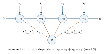
The transport result has a simple interpretation. An antitriplet can form a singlet with either of two neighbouring triplets. A handoff changes which pair is the singlet, leaving an unpaired colour carrier. These two pairing alternatives are not orthogonal. After orthogonalising them, their interactions are ordinary two-by-two matrices coupled to the internal clock. The remaining colour states are spectators only to the singlet contractions: they still evolve and interfere at measurement. At finite gap, excursions outside the selected cluster representation also return amplitude and phase. Keeping those returns exactly gives a memory law, rather than another adjustable coupling.
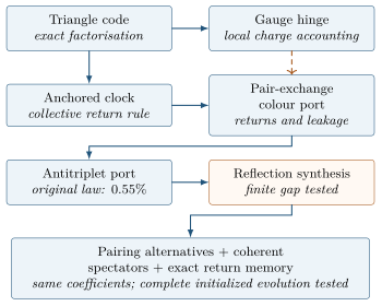
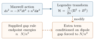
Figure 1. The construction and its compact description. The lower box rewrites the same synthesized Hamiltonian; it introduces no new fit. Calibrated couplings and dressed preparation remain inputs. The gauge-hinge and colour-port calculations are modules, not one fully integrated microscopic theory.
Readers interested primarily in transport can begin with the pairing algebra in Section 6 and its complete finite-gap law in Section 7. The earlier sections supply the ingredients: triangle algebra in Section 2, gauge coupling in Section 3, clock selection in Section 4, and pair-exchange ports in Section 5. The weaker inherited transport benchmark is retained to explain why correcting the colour representation required a new synthesis. The subsequent pairing reformulation holds that synthesis fixed.
1.1 Relation to previous work
Hamiltonian lattice gauge theory provides the language of links, electric energies and local Gauss constraints [1–3]. Finite-dimensional gauge magnets and quantum link models provide precedents for quantum registers carrying gauge variables [4, 5]. The three-qutrit code is standard [6–8]; the use of stabilizer constraints is not a new identification of error correction with gauge symmetry.
Two recent comparisons are particularly relevant. Lacambra et al. construct Gauss-law and vacuum codes for Abelian lattice gauge theories, explicitly distinguishing their code spaces and error sets [9]. Our finite Z3 constraints fit within that broader connection; the question here is the compatibility of specified clock and colour ports with them. Herbert, Gross and Newman construct qutrit codes inside SU(3) representations, with inherited finite Heisenberg symmetry [10]. Here we instead start with a three-register stabilizer code, then use permutation multiplicity spaces to encode a neutral clock alongside a colour carrier. Neither construction licenses identifying an arbitrary syndrome with physical colour.
Clock-controlled operations and perturbative simulation of many-body terms have established antecedents [11–14]. We use ordinary Schrieffer–Wolff and partitioning methods [15–17]. The contribution is the specific algebra, the complete denominators and the failure tests of these finite qutrit modules. No claim of priority is made for these general methods, or for a comprehensive microscopic theory of matter.
1.2 Notation and levels of evidence
We set ℏ=1. All register indices start at zero. A physical pair SWAP is Wij; it exchanges two fundamental qutrits. Π always denotes a projector. The symbols SX,SZ are reserved for triangle stabilizers. The encoded clock is τ, its mediator is m, and C denotes a cyclic permutation of three colour registers. A syndrome is the eigenvalue of a stabilizer, not an SU(3) representation label.
Table 1. Notation chosen to keep register roles, projectors and permutation operators distinct.
Symbol
Meaning
X,Z,ω
Qutrit shift, phase, and e2πi/3
XL,ZL
Logical Weyl pair on the triangle
(TZ,SZ),(TX,SX)
Two virtual syndrome Weyl pairs
Ψk,Vm
Individual hinge operator and coherent Fourier combination
Wij,Σn
Physical pair SWAP and its internal class sum
B21,D21,A21
Clock transition, imbalance and antisymmetric transition
Vλ,Rλ
Permutation multiplicity and SU(3) representation spaces
KBX
Singlet contraction between an antitriplet and a triplet
σx,σz
Two-by-two matrices on the pairing alternatives
Ar,Br,Dr
Retained, coupling and omitted blocks in colour sector r
Σr(z),Kr(t)
Exact return operator and time-domain memory kernel
Analytic identities below follow from the stated algebra. Finite matrix calculations corroborate them and evaluate dynamics at particular couplings. A check count records consistency of the implemented tests, not a theorem about an untested network. Numerical ranks and long-time probabilities are reported at their demonstrated precision. Appendix I identifies the evidence and retained numerical qualifications.
2 A triangle: logical information and two syndromes
2.1 Three physical qutrits, three virtual factors
Let X∣q⟩=∣q+1mod3⟩ and Z∣q⟩=ωq∣q⟩, so ZX=ωXZ. On three registers the commuting stabilizers are
SZ=Z0Z1Z2,SX=X0X1X2,[SZ,SX]=0.(1)
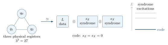
Their joint eigenvalues give nine syndrome sectors, each of dimension three. The common +1 eigenspace is the code. Thus a syndrome says which sector the state occupies, while a logical qutrit stores information within that sector.
An explicit factorisation is more useful than dimension counting. Choose
XL=X0X1†,ZL=Z0†Z1,TZ=X2,TX=Z0Z1.(2)
Each of (XL,ZL), (TZ,SZ) and (TX,SX) obeys the Weyl relation, and operators belonging to different pairs commute. They therefore generate three independent full matrix algebras:
(C3)⊗3≃HL⊗HsZ⊗HsX.(3)
This is a change of quantum coordinates, not three additional physical particles. Appendix A gives the inverse map and proves completeness. In particular, TX cannot globally be replaced by Z2†: that operator fails to commute with TZ=X2.
Figure 2. A triangle has three physical registers and a 27-dimensional space. Its virtual factorisation separates logical information from the two syndrome labels. The code is one three-dimensional sector; the displayed excitation energies are schematic. The Hamiltonian supplies the gaps.
Take ∣0L⟩=3−1/2(∣000⟩+∣111⟩+∣222⟩) and ∣qL⟩=XLq∣0L⟩. The resulting [[3,1,2]]3 code detects an arbitrary error on one qutrit and corrects one known erasure. Distance two does not mean that it corrects an arbitrary unknown one-qutrit error. Nor does the algebra supply an autonomous cooling or repair process.
2.2 Why the syndrome is not colour
The stabilizers commute with permutations of the three vertices. They do not commute with the full collective SU(3) action. With fundamental generators ta=λa/2 and Ta=∑j=02tja, the correctly normalised quadratic Casimir is
C2=a=1∑8TaTa=3I+W01+W12+W20.(4)
The identity follows from ∑atiatja=(Wij−I/3)/2[18, 19]. It is the Casimir, rather than each generator, that commutes with the stabilizers.
This distinction has a visible consequence. The antisymmetric state
∣ϵ⟩=2∣1L⟩−∣2L⟩(5)
is an SU(3) singlet. The code-space Casimir spectrum is {0,6,6}, not a scalar. A colour-symmetric interaction and a syndrome-preserving interaction are different requirements. Later sections introduce an actual colour representation and track it separately.
2.3 A gapped triangle and its hinge channels
Define syndrome projectors
ΠZ=I−3I+SZ+SZ2,ΠX=I−3I+SX+SX2,(6)
and a vertex cycle R△=W01W12. A useful Hamiltonian is
All coefficients are real, with positive excitation gaps in the regimes used here. The two surrounding projectors matter: they make the bracket act only on excited Z-syndrome sectors, leaving the code energy zero. Dropping them would split the logical states before any hopping was introduced.
They commute with SX and raise the SZ eigenvalue by ω. Their noncommuting Weyl relations belong to the qutrit Heisenberg group of order 27, commonly denoted Δ(27). This finite algebra is not the full continuous colour symmetry.
Each Ψk is unitary, so it has no dark vector, even when its input is restricted to the code. The rank-one objects are instead the coherent sums
Thus the three coherent channels together cover the whole logical space. The channel labels must follow the chosen orientation of R△. Reversing that cycle reverses the sign of δ in the energy table; it does not change the physics if done consistently.
For example, let dj be the excitation energy with R△ eigenvalue ωj in the reached syndrome sector:
d0=ΔZ+6μ,d1=ΔZ+3μ+δ,d2=ΔZ+3μ−δ.(11)
An incoherent sum over three orthogonal, equally coupled one-endpoint link channels gives the positive return kernel
Θ1end=m=0∑2d−m+ΔE3J2∣ℓm+1⟩⟨ℓm+1∣.(12)
Here ΔE is the link excitation cost; it may be absorbed into the definition of the denominator. The energy correction is −Θ1end. A positive return kernel is not a derivation of a positive fermion mass. Equation (12) also assumes an electric reference state for which distinct link excitations are orthogonal; merely setting an inter-link coupling to zero does not specify that state.
3 Gauge constraints on the face graph
3.1 Geometry organises the registers
The supplied oblate cell has vertices
±(21,21,0),±(21,−21,0),±(0,0,21).(13)
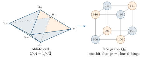
Its polar-to-equatorial semi-axis ratio is 1/2. Each triangular face chooses one vertex from each antipodal pair, giving a label f∈{0,1}3. Two faces share an edge precisely when one bit differs. The face graph is therefore the cube graph Q3: eight nodes, twelve edges and three edges incident on each node.
Figure 3. The supplied oblate cell and its cube face graph. An edge of the graph represents a shared hinge, not a new spatial cube. Node labels identify the eight faces by antipodal choices; fill distinguishes even and odd parity. Three qutrits belong to each face independently, and one belongs to each link: 36 registers before clock or colour auxiliaries. Drawing adjacent faces does not identify their registers.
This ownership convention is essential. It differs from placing a single shared qutrit at each of the six geometric vertices. All subsequent tensor products use independent face registers. The even and odd extended face planes bound tetragonal disphenoids, not regular tetrahedra; the geometric comparison with Sommerville’s tetrahedra is ancillary [20]. The Clifford sign convention on the face graph is recorded in Appendix C; it alone establishes neither fermionic exchange statistics nor a continuum limit.
3.2 A gauge-invariant hinge
Orient each link e=(f,g) and give it a Weyl pair (Ue,Ee) with EeUe=ωUeEe. Let σ(f,e)=+1 at the outgoing end and −1 at the incoming end. Define
Gf=SZ,fe∋f∏Eeσ(f,e).(14)
Together, the eight Gf and eight SX,f commute. The gauge constraint selects their specified eigenvalues. For a hinge of type k,
commutes with every one of those constraints. At f, the matter phase ω−1 is cancelled by the link phase ω; at g the inverse cancellation occurs. This is a local charge-accounting identity, not a numerical approximation.
In contrast, Ue†Ue′ for two links meeting at f cancels the phase at f but changes the constraints at their remote endpoints. Conserving total link flux at a junction is weaker than conserving every local Gauss law. We do not add such bare inter-link mixing.
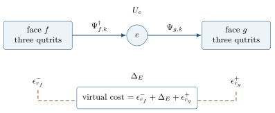
Figure 4. A virtual hinge excursion excites both endpoint triangles and the link. Its denominator contains three energy costs. Either orientation must return, and both contribute to the second-order energy shift. The figure shows one hinge; three hinge types on Q3 lead to three different neighbours.
3.3 Both ends contribute to the denominator
For the convention of Eq. (7), the states Ψk∣ℓr⟩ and Ψk†∣ℓr⟩ have energies
It depends on the partner’s logical state. The baseline cost is 2ΔZ+ΔE, not ΔZ+ΔE. This is the simplest example of the complete-background rule used throughout the paper: pay for every excitation present in the intermediate state.
The source’s three-channel two-endpoint comparator is 3θe for equal couplings and identical endpoint spectra. That multiplier must not be attached to a single edge of Q3. The network return is a sum over its actual edges and their partner states. In addition, Eq. (17) is a virtual return inside the code; a positive diagonal return does not itself demonstrate real charge transport between faces. The gauge module also has multi-register vertices, so it is not already a strictly pair-local implementation.
4 An anchored clock that restricts returned operations
The clock is intended to prevent an incomplete set of ports from mimicking a completed collective transition. This is a selection rule on returned processes. It does not require a programmed time sequence, but it does require a specified Hamiltonian, a prepared reference state and energy penalties.
4.1 The complete five-qutrit law
Use mediator qutrits m0,…,m3 and a syndrome qutrit c. In the computational basis, let
The last line contains the two supplied three-body pins. Their role is concrete: they relate mediator changes to syndrome changes, so the independent port phases cannot all be removed at once.
Figure 5. The anchored clock. Solid bonds are diagonal mismatch penalties; dashed three-register couplings are the supplied pins in Eq. (19). Without these pins, independent phase changes remove the port labels and all sectors have the same spectrum.
To check it, use ZaXZ−a=ωaX. The first three single-port phases cancel, the fourth becomes s, and the phase of each pin is zero modulo three. The background is diagonal and unchanged. The all-zero reference state is fixed by U.
Consequently, a reference-to-reference amplitude depends on the four sector labels only through their sum. Its discrete Fourier expansion contains collective powers of the port product. This is the precise locking statement. It does not say that an auxiliary can never be excited, or that every allowed transition has a large amplitude. A ring with only the single-site terms in Eq. (19) has no such nontrivial selection: ∏aZmasa removes every phase. The revised text includes the missing pins explicitly.
4.2 Generating a pin with two-body interactions
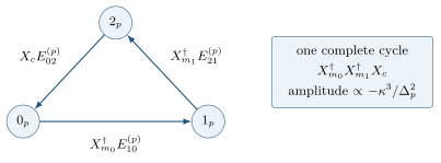
An auxiliary qutrit p can replace one supplied pin. Give ∣1⟩p and ∣2⟩p equal energy Δp, and define Eab(p)=∣a⟩p⟨b∣p. Take
Every term involves two physical registers. The directed virtual sequence 0→1→2→0 applies Xm0†, Xm1† and Xc in order. In the isolated equal-gap gadget,
The second-order return is scalar in this isolated problem. The third-order term is the desired pin. Replacing Xc by only ∣1⟩c⟨0∣c would define a different gadget; it is not the cyclic qutrit law checked in the source.
Figure 6. The pin compiler. A single static Hamiltonian supplies all arrows and their Hermitian conjugates; no external schedule selects their order. The auxiliary level determines which operator acts next. The displayed denominator assumes the isolated gadget; background bond and syndrome costs alter it in the integrated clock.
commute with VA. An analogous auxiliary with Xc† generates the second pin. This yields a seven-qutrit clock with pair-local terms. Once Eq. (18) is present, virtual energy costs depend on the intermediate mediator and syndrome states; Eq. (23) must not be reused as an exact integrated coefficient. The source retains those returns and checks the resulting sector conjugacies and perturbative limits.
For comparison, the earlier binary-mediator/qutrit-syndrome construction admits a fifth-order partial process: three syndrome shifts return a qutrit to itself, while three binary flips leave a flip. Matching the cyclic algebra removes this specific mismatch. This comparison supports the all-qutrit choice, not a claim that every hybrid architecture fails.
5 Colour ports: what pair exchange can implement
5.1 A neutral clock cannot control one colour register alone
For a neutral elementary clock p and a fundamental colour qutrit B, Schur’s lemma gives
EndSU(3)(Cp3⊗3B)=M3(C)p⊗IB.(25)
Indeed, p supplies three copies of the same irreducible colour representation. A commuting operator can mix those copies but must be scalar on each colour carrier. The commutator map on all 81 operator coordinates has rank 72 and kernel dimension nine, corroborating this argument.
A gate E10(p)⊗WBC is invariant when B,C are both fundamental, but it acts on three registers. Supplying such gates gives a useful conditional benchmark. It does not solve the pair-local problem. The way forward explored here is to encode the neutral clock in the multiplicity of a charged cluster, so a physical pair exchange can act jointly on clock and colour.
5.2 A joint return rule with supplied colour gates
Before compiling the colour interface, one can connect the seven-qutrit clock to a logical register L, three fundamental colour registers A,B,C, and an auxiliary pC. The resulting twelve-qutrit Hamiltonian is static but includes the three-body colour gates just described. Its useful property is an exact selection rule, not an inferred high transfer probability.
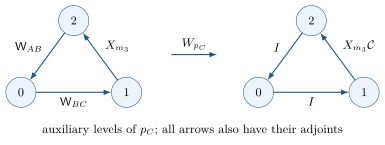
Define C=WABWBC. Dressing auxiliary level one by WBC and level two by WAB moves both exchanges onto the middle clock step (Fig. 7). In sectors XL=ω−sL and C=ω−sC, the integrated clock has port labels (sL,sL,−sL,sC). Their sum is sL+sC. Because the locking transformation fixes the mediator–auxiliary reference state, its return operator has the form
This follows by Fourier expansion of a function on Z3: the returned operation can depend only on the joint eigenvalue. Charge-only and colour-only terms are excluded from this conditional return. The functions aj(t) need not give perfect transfer, and the unconditioned state can retain auxiliary excitation.
Figure 7. The supplied colour port before and after a change of basis. Dressing levels one and two by the two SWAPs concentrates their product on the middle step. This is an exact representation of the same Hamiltonian, not a physical gate sequence or a reduction of its register support.
Equation (26) requires no logical ∣2L⟩⟨2L∣ penalty: that penalty does not commute with XL. A high transfer probability from a separate detuned port therefore does not carry over. Appendix B states the full conditional law and its sector dimensions. The next step is to replace its supplied colour gates by microscopic pair exchanges without losing these constraints.
5.3 A four-qutrit cluster encodes clock and colour
Schur–Weyl duality separates tensor powers into colour representations and permutation multiplicities [19, 21, 22]:
(C3)⊗n=λ⊢n,ℓ(λ)≤3⨁Rλ⊗Vλ.(27)
Colour rotations act on Rλ; pair exchanges act on Vλ. For four fundamentals,
The subscripts are total dimensions, summing to 81. The pair Hamiltonian
H4(0)=Δ4(2I+Σ4),Σ4=0≤i<j≤3∑Wij,(29)
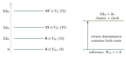
has energies 0,2Δ4,4Δ4,8Δ4 in these sectors. Its nine-dimensional ground space W4≃Hτ⊗3B therefore supplies a neutral encoded clock and a genuine colour carrier together.
Here B21 changes the active clock level, whereas D21 measures its imbalance. They are not interchangeable. The antisymmetric transition is A21=21[D21,B21]=E21(τ)−E12(τ).
Adding external fundamental qutrits A,C gives six physical qutrits. Signed combinations of exchanges between the cluster and those registers project to
Appendix D lists the physical pair formulas. This is an exact first-order projection, not an assertion that the full interaction preserves W4.
Figure 8. Cluster energies and the complete virtual cost. A port leaving the reference clock excites both the cluster and the clock penalty, so the relevant denominator is 4Δ4+Δτ. The additional clock cost cannot be omitted merely because the port is written using cluster exchanges.
5.4 Virtual returns and a physical locality test
From τ=0, the two port leakage vectors lie in the cluster sector of energy 4Δ4 and have an additional clock energy Δτ. Their second-order return is
It is cancelled on the 27-dimensional reference space by the pair counterterm
Hct=9(4Δ4+Δτ)10κC2i=0∑3(WiA+WiC).(33)
This is a perturbative cancellation on a specified subspace. It does not remove every instantaneous return of a bare initial state. At Δ4=32, replacing the incomplete denominator 4Δ4 by the full one reduces the source’s colour-cycle harmonic error from 10.70054% to 0.09834%. The source also reports 99.2178% target transfer in a separate two-step six-qutrit diagnostic; its different Hamiltonian and readout time must not be combined with the later eight-cluster result.
Coupling a mediator m to the encoded clock through
Vmid=−2g[(Xm+Xm†)B21+(Xm−Xm†)A21](34)
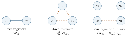
is Hermitian: the second product contains two commuting skew-adjoint factors. Nevertheless, A21 is a sum of three-cycles on physical registers. Multiplying it by a mediator operator produces four-register support.
Figure 9. Physical support, rather than the number of encoded symbols, determines interaction order. A pair SWAP is two-body; an elementary clock-controlled SWAP is three-body; a mediator times a three-register cluster operator is four-body. The dashed shapes denote supplied higher-body terms, not decompositions into independent edges.
A useful test takes the trace against a product of traceless operators on the proposed support. Any term missing one of those registers gives zero trace. Nonzero witnesses of 3/4 for A21, −9/4 for Vmid/g, and 27/2 for the relay vertex certify three-, four- and four-register support respectively. Definitions appear in Appendix D.2. Rewriting a product in terms of SWAP symbols does not reduce that support.
5.5 A relay works conditionally, with its full background
A relay auxiliary r gives a further benchmark, still with supplied higher-body vertices. The relevant intermediate energy above the reference is Δr+Δτ=24, rather than Δr=16. The 810-state calculation uses the same Hamiltonian at two proposed readout times. At tisolated=32tcomplete it gives 74.7840% target transfer; at tcomplete it gives 99.8836%. Thus the comparison tests the timing formula, not two different physical laws.
The Hamiltonian includes a clock-return counterterm 3κr2Π12(τ)/(Δr+Δτ)=0.02Π12(τ). Removing it gives 99.8762% at the complete time. Table 2 includes the previously omitted population so that its categories close.
Table 2. The supplied eight-register relay benchmark. The remainder is obtained by subtraction using the recorded table values, so the final digits are rounding-dependent. These are populations at two times, not a sampled transfer curve.
Probability category
tisolated
tcomplete
Target
0.74784045
0.99883583
Initial
0.25132920
0.00000171
Reference clock, wrong colour
2.79002210−4
5.40424110−4
Other reference states (remainder)
7.1909410−5
5.5830010−6
Active clock, r=0
4.78714610−4
6.15342910−4
Relay excited
5.89212310−7
9.41137310−7
Outside W4, r=0
1.34621410−7
1.68861910−7
Near-degenerate levels create a separate readout issue. The earlier nine-point spectral readout averaged doublets at three points but selected one branch at two others on an overlap margin of about 5×10⁻⁸. Its very small Fourier harmonics depend on that inconsistent convention. Keeping the full six-state low-energy colour space and using polar projection instead gives a leading cycle coefficient −1.56146305×10⁻⁵. Appendix E explains the construction and distinguishes the diagnosed double-quadrature case from an incompletely diagnosed control.
The seven-fundamental sector λ=(3,2,2) carries a triplet, with 21-dimensional multiplicity and physical dimension 63. Its nine-dimensional clock–mediator multiplicity subspace splits from two six-dimensional complements. Pair exchanges generate a symmetric clock–mediator quadrature at first order; virtual processes also generate the desired antisymmetric quadrature and additional returns.
The return operators are not freely adjustable within the available first-order pair span. The measured span ranks rise from 20 to 23 on the nine-dimensional space, and from 11 to 14 on its six-dimensional active-clock part when the three channel returns are appended. The weighted-return test gives 11 to 12. These finite numerical ranks concern the stated ansatz and channel matrices. They are not a no-go theorem for all pair-exchange Hamiltonians.
The colour ports further carry a representation factor
Fm=23Πs−163Πe=83I+169(Xm+Xm†),(35)
where Πs=(I+Xm+Xm†)/3 and Πe=I−Πs. A matched symmetric interaction corrects its unequal weights. The formerly quoted 98.9196% transfer, however, also uses a supplied antisymmetric interaction and a spectrum-calibrated correction
3δE(W45+W46+W56),δE≃1.981765×10⁻⁴.(36)
Without that calibration the target probability is 5.3166%. It is therefore a calibrated conditional benchmark, not a parameter-free result.
The historical Models C and D used an incomplete active-state resolvent. Their recorded probabilities remain reproducible, but their interpretation as evidence that physical pair returns destroy transport has been withdrawn. The full background introduces additional denominators 264 and 520 alongside −8,248,512. Model E is a different bare one-point diagnostic, not a general impossibility result. We retain these distinctions rather than presenting an unqualified five-row success/failure table.
6 Colour transport and the pairing algebra
6.1 A larger cluster changes the colour algebra
The eight-fundamental sector λ=(3,3,2) has Dynkin labels (0,1): it carries 3ˉ, not 3. Its multiplicity dimension is 42 and its physical dimension is 3×42=126. With two external fundamentals the projected space is
V332⊗(3A⊗3ˉB⊗3C),dim=42×27=1134.(37)
This representation change is decisive. A label swap between two triplets commutes with their collective colour rotation. A label swap between a triplet and an antitriplet generally does not. In the latter case the invariant two-factor algebra is spanned by the identity and the singlet projector, since 3ˉ⊗3=1⊕8. This is the elementary mixed-tensor distinction underlying more general contraction algebras [23].
The fundamental generators act on the antitriplet as tˉa=−(ta)∗. All eight total charges commute with KAB and KBC. Their multiplication rules differ from those of SWAPs, which square to the identity. One cannot transfer a synthesized permutation Hamiltonian into this carrier by changing names alone.
6.2 Two pairing directions and their spectators
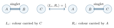
The mixed colour problem admits a small exact algebra. For each remaining fundamental colour c, define the two normalized singlet-pairing states
They describe which adjacent pair is a singlet while the third register carries colour. Their span has dimension six. Both contractions annihilate its 21-dimensional orthogonal complement. In representation language,
3⊗3ˉ⊗3=(3⊗C2)⊕6ˉ⊕15.(40)
The two-dimensional factor records the pairing alternative; it is not a replacement for the fundamental colour carrier. A symmetric choice of orthonormal coordinates makes both ports equally simple:
∣+⟩c=8/3Lc+Rc,∣−⟩c=4/3Lc−Rc.(41)
Write σx and σz=diag(1,−1) for the Pauli matrices on this pairing factor. They are distinct from the physical qutrit Weyl operators X,Z. In these coordinates,
KAB=(2221),KBC=(2−2−21),WAC=σz.(42)
The common diagonal part distinguishes symmetric from antisymmetric pairings. The off-diagonal parts mix them with opposite signs. These matrices obey KABKBCKAB=KAB and the mirror relation, as well as K2=3K. The order of the two contractions is therefore retained, not averaged away.
Figure 10. Two alternatives in colour Hilbert space. In Lc the AB pair is a singlet and C carries colour; in Rc the BC pair is a singlet and A carries colour. Their overlap is 1/3, so a handoff is a coherent change of pairing, not an exchange of two classical bonds. The drawing denotes representation factors, not physical distance.
6.3 The physical port is fixed by two independent conditions
Let Pu be the external transposition represented on the nine-fundamental singlet multiplicity V333, and set Mu=(I−3Pu)/4. Write the projected external SWAP as
Π332WuXΠ332=Au⊗I+Bu⊗KBX.(43)
On the singlet, K has eigenvalue three, so Au+3Bu=Pu. Independently, tracing over the external fundamental gives 3Au+Bu=I. Solving these two equations yields
Au=31I+61Mu,Bu=−21Mu.(44)
For the signed ports G10,C=W0C−W1C−W2C+W3C and G02,A=W0A−W1A+W2A−W3A, the identity coefficients cancel, leaving
Π332GaXΠ332=Ma⊗(61I−21KBX).(45)
Cancelling the colour-identity term requires an internal counterterm −Ma/6 per unit port coupling. This is a chosen cancellation condition, not a unique consequence of colour invariance. The previous permutation surrogate used +Ma/3. Section 6.7 considers a different invariant choice which makes the colour factor a reflection.
With HI denoting the full retained internal Hamiltonian, including its small mediator penalty, the corrected projected law is
All coefficients are real, and all displayed factors are Hermitian. The two colour contractions generally do not commute. Both are retained in the dynamics.
6.4 What the high-fidelity benchmark actually tested
Before this correction, 17 internal pair-exchange coefficients were numerically selected to satisfy 15 target conditions on zero-energy Schur complements in a 252-state model V332⊗C[S3]. That finite-dimensional permutation surrogate gives 99.9651% target transfer. It is a valid Hamiltonian synthesis calculation in its declared space, but it is fitted to a desired effective operation. It is not a dynamically selected coupling law and not the physical mixed-colour interface.
The synthesis retains all its off-diagonal blocks. Its prepared reference is dressed, rather than the bare seven-cluster reference: the initial dressed state has 6.8491% weight outside the bare nine-dimensional space. Four odd cross-exchange operators act out of the five-dimensional reference sector even though their projection within it is zero. These support qualifications matter when defining leakage.
For the comparison below, the 17 coefficients are held fixed. So are Δτ=8, κC,eff=gmid=0.05, cport=−16κC,eff/3, and the third-order readout time
Holding the inherited coefficients fixed is a useful test of the representation correction. It does not undo their original synthesis to the permutation target.
6.5 A forbidden target and an allowed but weak transition
Use integer-scaled diagonal weights t3=diag(1,−1,0) and t8=diag(1,1,−2). A colour state ∣a,bˉ,c⟩ has total weight
q(a,bˉ,c)=t(a)−t(b)+t(c).(48)
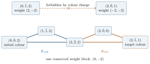
The old transition (0,1ˉ,2)→(2,0ˉ,1) changes this weight from (2,−2) to (−2,−2). Its amplitude is exactly zero for all times under Eq. (46). In fact both contractions annihilate the initial all-distinct colour state.
Figure 11. Conserved colour weight distinguishes the two tests. The old permutation target crosses weight sectors and is forbidden. The repaired test stays in the complete five-colour block of weight (0,−2). Contractions join the two indicated triples through (2,2ˉ,2); they are coherent rank-one operators on each triple, not deterministic swaps.
An allowed test starts in (0,0ˉ,2) and targets (2,1ˉ,1), while the dressed mediator changes from zero to one. The entire weight block is
Keeping all 42 internal states gives a 210-state dynamical calculation. No additional coupling or time was fitted after changing the colour algebra.
Table 3. The corrected physical readout. The five categories are disjoint and sum to one before rounding. Decimals identify the saved calculation; they are not a claim of accuracy in every digit. The justified description is about 0.55% target transfer. The forbidden old target is an analytic zero, not another population in this table.
Repaired physical model at tπ
Probability
Allowed target
0.005455164694
Initial state
0.111333946718
Other dressed reference states
0.883145915170
Active clock within dressed nine-space
1.43883×10⁻⁸
Outside dressed nine-space
6.49590×10⁻⁵
The source and an independently assembled SciPy calculation differ by at most 2.991×10⁻⁶ in the population distribution. That narrowly fails the declared 2×10⁻⁶ comparison tolerance and remains a failed check. A common-matrix Rayleigh-quotient diagnostic reduces the difference below 10−6; a floating-point residual bound contains the original discrepancy. Neither diagnostic converts it into a rigorous interval certificate or retroactively changes the tolerance.
The physical conclusion is stable at that precision: there is nonzero colour rearrangement, but no high-fidelity transfer at this point. No masses or mixing angles were fitted or predicted.
6.6 Why spectator interference matters
In the five-colour block, write TA=(∣+⟩2,∣−⟩2) and PD=I5−TATA†. Equation (46) splits into one 84-state active block and three identical 42-state spectator blocks. Its complete propagator is
Spectators still evolve internally. Their amplitudes must be added coherently at readout. An exact basis check and comparisons of all 210 amplitudes at 65 fixed times reproduce the saved calculation within its numerical precision; five complete-propagator comparisons also test initial states outside the prepared support. At tπ, the maximum population difference is 1.87×10⁻⁶. The earlier independent tolerance failure remains unchanged. In particular, dropping interference predicts 36.24% in the initial state rather than the correct 11.13%.
This interference also corrects a proposed bound. For i=(0,0ˉ,2) and f=(2,1ˉ,1),
Thus 9/64 bounds the active contribution alone; it is not a universal bound on the complete probability. For Hamiltonians generated by internal operators tensored with I,KAB,KBC, the combined amplitude is bounded by 3/8+1/8=1/2, giving P≤1/4. This bound is attained: the colour Hamiltonian KAB+KBC at t=π/2 has amplitude 1/2 between these two states. An independent internal swap can simultaneously change the internal label. The bound concerns this contraction-generated class, whose dark colour sector has a common internal evolution; it is not asserted for every invariant interaction.
6.7 Synthesizing transport with singlet reflections
A different counterterm gives a useful physical benchmark. Adding +7Ma/12, instead of cancelling the identity term, changes Eq. (45) to
This is an invariant singlet reflection realizable through the same physical port and an internal pair-exchange correction. Two such reflections do not obey the S3 braid relation. On the active doublet their product has eigenvalues (−7±4i2)/9, and their commutator has eigenvalues ±8i2/9. Treating them as ordinary transpositions would give the wrong dynamics.
In the pairing coordinates of Eq. (41), the same statement is especially transparent:
The two reflections have a common pairing-diagonal component and opposite mixing components. Their noncommutation is part of the transport law.
The new benchmark solves zero-energy Schur-complement targets again, using 17 supplied coefficients xphys and the reflection port scale 3cport/4. Its projected Hamiltonian is
The actual readout time remains Eq. (47), 256000π, rather than a new representation-rescaled time. The preparation and measurement use the corresponding dressed internal reference states. All reported transitions below change the dressed mediator from zero to one. No masses or mixing angles enter the synthesis, but the couplings are selected to implement a target operation; they are not dynamically derived.
Table 4. Independent reconstruction in the complete 210-state colour-weight block. The last two rows reverse only the colour endpoints: the internal transition remains 0→1, so they are not time-reversed experiments. The supplied extension had interchanged these colour labels. The 14.06% value is not saturation of a universal 9/64 ceiling.
Projected physical transition at tπ
Probability
Singlet pairing L2⟶R2
0.9998093
Computational (0,0ˉ,2)⟶(2,1ˉ,1)
0.0851880
Computational (2,1ˉ,1)⟶(0,0ˉ,2)
0.1405992
The singlet handoff gives approximately 99.9809% target probability. The residual budget is 7.65×10⁻⁶ in the initial state, 1.20×10⁻⁵ in other dressed reference states, 1.71×10⁻⁶ in the active clock, and 1.69×10⁻⁴ outside the dressed nine-space. The complete handoff state independently agrees with the supplied reduced calculation within 2.79×10⁻⁶ in Euclidean norm. The spectator Hamiltonian is now HI+43cport(M10+M02), rather than HI; a high survival probability at one time is not exact freezing.
7 The complete pairing law at finite gap
The projected pairing algebra is exact within the selected representation. Physical exchanges can also visit other representations when the penalty is finite. This section keeps those visits without replacing their effect by fitted constants. The result is a compact law for the reference amplitudes, with an exact memory kernel and coherent spectator reconstruction.
7.1 The fixed microscopic law and its representation penalty
External physical exchanges can leave the eight-cluster representation. The previous squared omitted-sector leakage trace, 162, is an operator diagnostic rather than a time-evolved probability. A finite penalty now allows those states and their returns to be retained explicitly.
Let Σ8=∑0≤u<v<8Wuv. On eight fundamentals its content-sum spectrum is
Spec(Σ8)={0,2,4,7,8,10,12,14,20,28}.(55)
Only the (3,3,2) representation has eigenvalue zero. Thus Δ8Σ8/2 is a positive semidefinite pair-exchange penalty selecting that representation, with a 126-dimensional ground space, not a unique ground state. The first two representation gaps are Δ8 and 2Δ8.
For singlet-pairing preparation the total colour is fundamental. Its ten-qutrit permutation multiplicity is V433, and restriction to the eight-cluster part gives
V433↓S8=V332⊕2⊕V422⊕V431,210=84+56+70.(56)
These 210 states differ from the earlier 42×5 charge block. They include all 126 omitted states accessible within this conserved total-colour sector. The external exchange WAC is −I on V422 and +I on V431. The total fundamental colour supplies an additional threefold degeneracy on which the invariant Hamiltonian acts trivially.
The single-port numerator identities are collected in Appendix G. They constrain individual returns but do not replace the complete intermediate Hamiltonian or its mixed-port couplings.
The simulated finite-gap Hamiltonian includes all corrections actually used:
The Ma here are their internal pair-exchange lifts; the Oj are six existing internal exchange combinations. Both δcj and δAC are computed separately at each gap from a six-reference-state Schur complement. Their numerical values are supplied with the verification data. They are essential parts of the synthesized law, not merely bookkeeping: omitting the six internal corrections lowers the transfer at Δ8=25600 from about 91.69% to 82.04%.
Table 5. Independent pair-exchange reconstruction and real-time evolution in V433, retaining all 210 multiplicity states. Numerical probabilities agree with the replayed source within 2×10⁻⁵; the displayed digits are diagnostic. The first three rows use two-body terms. The last row additionally imposes a representation-dependent gap shift and is not a purely two-body construction.
Finite-gap handoff at tπ
Target probability
Omitted population
Δ8=25600, all corrections
0.91694
4.06×10⁻¹⁰
Δ8=102400, all corrections
0.99582
2.92×10⁻¹¹
Δ8=102400, δAC=0
0.87474
2.88×10⁻¹¹
Δ8=25600, modified 5/6 gap ratio
0.99649
7.14×10⁻¹⁰
For the ratio control, an additional term −(7/6)Δ8Π431 changes the second omitted gap from 2Δ8 to 5Δ8/6. It tests the return identity in Eq. (92); a microscopic pair-local realization of this selective shift has not been provided. In the first three rows, all terms are physical pair exchanges plus scalar offsets. The data establish a finite-gap transport construction for a prescribed preparation and synthesized coefficients. They do not demonstrate autonomous preparation, error repair, stability under arbitrary perturbations, or selection of those coefficients by an underlying law.
7.2 Two pairing operators, with all coefficients held fixed
We now rewrite Eq. (57), rather than synthesize another Hamiltonian. Define the internal sum and difference of the ports and retain all six calibrated corrections:
This is the compact transport law: internal evolution, a pairing-diagonal interaction, and a pairing-mixing interaction. The 42-dimensional internal matrices are unchanged. The two-by-two factor describes which pair is a singlet, while the unpaired fundamental colour remains present. Equation (59) is a coordinate identity, not an adiabatic approximation.
The same law explains the spectators. The contractions vanish on them, but each reflection acts as the identity. Their reference Hamiltonians are
The different signs come from the external exchange parity. At infinite penalty with the calibrated corrections set to zero, the three spectators again share one internal Hamiltonian. At finite penalty their return kernels also depend on their conserved total-colour sector.
7.3 The three spectators enlarge the finite-gap calculation
The earlier V433 calculation tests a prepared singlet pairing. A computational colour state contains additional total-colour representations. Preserving its interference requires retaining those sectors too, under exactly the same physical pair-exchange law.
In the five-colour order Bcol, an orthonormal spectator basis is
The minus mode belongs to 6ˉ; the two plus modes span the selected weight space in 15. Invariance makes the two 15 copies evolve identically. This degeneracy follows from the colour representation, not a newly imposed relation between coefficients.
Table 6. Blocks needed at the selected total colour weight. “Retained” means the eight-cluster (3,3,2) sector, including all its internal states; it is larger than the dressed preparation space. The two 450-state copies share one propagator.
Total colour
Young shape
Full block
Retained
Omitted
Copies
3
(4,3,3)
210
84
126
1
6ˉ
(4,4,2)
252
42
210
1
15
(5,3,2)
450
42
408
2
The resulting initialized sector has 210+252+2(450)=1362 states: 210 retained and 1152 omitted. Only three distinct diagonalizations are needed, the largest of size 450. This is the full sector reachable from the declared cluster-representation preparations, not all 310 physical-register states. Tableau and weight-multiplicity counts check the dimensions independently.
For example, ∣0,0ˉ,2⟩ has weights 3/8 in the active pairings and 1/4,1/4,1/8 in the three spectators of Eq. (61). All four channels contribute. On returning to the original reference basis, one sums their complex amplitudes before squaring. This retains all six pairwise interference terms; the sector decomposition is not a measurement that destroys their coherence.
7.4 Exact returns are a memory kernel
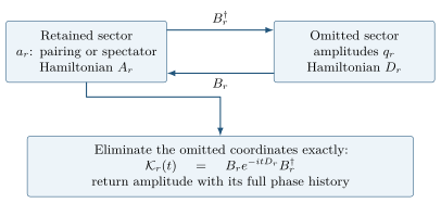
For each conserved colour sector r, partition the full Hamiltonian into retained and omitted states:
Equations (59) and (60) supply Ar. The physical ports supply Br. Crucially, Dr is the whole omitted-sector Hamiltonian: representation penalties, internal background, calibrated terms and noncommuting couplings between omitted representations. Replacing it by a bare gap would change the law.
Block elimination, the same partitioning principle used earlier [16], gives the exact return operator
where Pr restricts to retained coordinates and the inverses are taken where defined. The dependence on z is essential: different spectral components acquire different return amplitudes and phases. No parameter is adjusted to achieve this equality.
The time-domain version is equally informative. Integrate the equation for qr and substitute it into the equation for ar:
The kernel describes amplitude leaving the retained space, evolving in the other representations, and returning later. The middle term accounts for any omitted amplitude present initially; it vanishes for the declared reference preparations. The omitted amplitude itself is reconstructed by
Thus the complete state is retained, not just a normalized projection onto the reference space.
Figure 12. Exact partitioning within each conserved colour sector. A virtual excursion can return with a different phase even when very little population remains in the omitted space. The retained pairing and spectator amplitudes are recombined coherently at readout. The time kernel represents the full omitted dynamics; it is not a new reservoir or an entropy sink.
For numerical evaluation we diagonalize Dr=VrΩrVr†, set Cr=BrVr, and evolve the Hermitian auxiliary-mode matrix
(ArCr†CrΩr).(66)
Every mode is retained, and its frequency and coupling come directly from the fixed Hamiltonian. This realizes the exact memory law without discretizing the convolution. It simplifies the algebra and separates the mechanisms, but does not reduce the exact number of dynamical modes.
7.5 Full-evolution comparison without refitting
The comparison fixes the original 17 coefficients, the six corrections and external correction for each accepted case, the dressed basis, and the time tπ. Seven preparations are tested: L2, R2, the computational colours (0,0ˉ,2) and (2,1ˉ,1), and the three spectators in Eq. (61), each with internal label zero. Their complete states are compared at 65 equally spaced times from zero to tπ.
The projected model and all four finite-gap cases in Table 5 are included. Five complete-propagator comparisons per distinct Hamiltonian give 65 comparisons in total. These also test arbitrary initial amplitudes in the included omitted sectors, not just the seven reference preparations. The reconstructed reference readout keeps every cross term, and all omitted amplitudes are retained in an orthonormal Young-sector basis.
Table 7. Comparison over the declared cases and time samples. The identity is exact algebraically; these are floating-point implementation discrepancies, not error bars on a physical prediction.
Full law versus pairing–memory formulation
Largest discrepancy
Hamiltonian reconstruction, maximum entry
8.23×10⁻¹¹
Retained resolvent, relative Frobenius norm
1.06×10⁻¹⁰
Seven prepared state vectors, Euclidean norm
8.99×10⁻⁵
Any sampled reference probability
1.74×10⁻⁵
Complete propagators, operator norm
1.89×10⁻³
All 60 registered checks pass. The unchanged 2×10⁻⁵ comparisons with the original handoff readouts also pass. Long evolution magnifies binary64 spectral and phase differences, especially for high-energy initial states. Numerical reconstruction and phase allowances contain the observed discrepancies; their largest amplitude allowance is 4.50×10⁻³, below the prospective 5×10⁻³ ceiling. No global phase alignment is used. This is numerical corroboration of the exact block identity, not machine-precision evolution or an interval certificate. The extension is constructor-checked and has not yet received an independent run review.
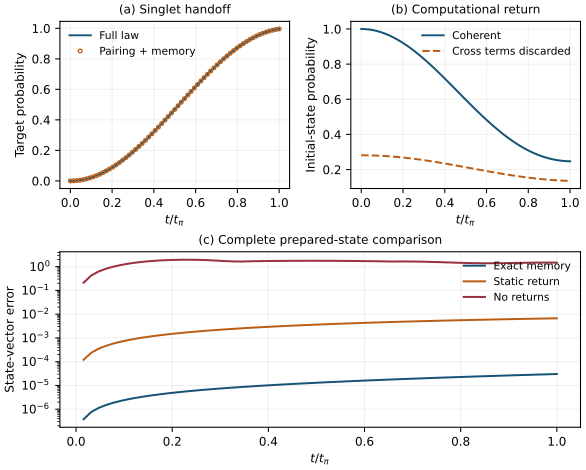
Figure 13. Saved time samples under the fixed law. (a) Full and compact singlet handoff at Δ8=102400. (b) Return to the initial computational state with and without coherent cross terms at that gap. (c) The largest full-state error among the seven preparations at Δ8=25600, comparing exact memory, a static return, and no returns. The 65 samples are connected as guides; the plot does not resolve every rapid oscillation.
The controls distinguish three ways a smaller model can lose the physics. Incoherent reference readout fails ten checks. Removing Br fails 32 and changes the lower-gap singlet handoff from 91.69% to 11.38%, with all calibrated terms still fixed. Replacing the return operator by Σr(0)=−BrDr−1Br† and decoupling the omitted modes fails 14. The latter gives a deceptively close lower-gap handoff, 0.916924 instead of 0.916936, and passes the near-zero-energy resolvent comparisons at their tolerance. Yet its largest prepared-state error there is about 0.00671, and it fails the complete complex-propagator test. This rejects that specified static replacement as an exact formulation, not every possible approximate effective Hamiltonian.
The spectator results explain why population leakage alone is insufficient. At the lower gap, their final initial-state survival probabilities are approximately 39.35% and 42.13%, while their omitted populations remain of order 10−9 on the sampled grid. Small instantaneous leakage can still accompany substantial accumulated virtual phase and internal motion. At the larger gap, coherent return to the computational initial state is 24.6915%; adding block probabilities instead gives 13.5400%. Its forward computational transition to (2,1ˉ,1) with internal label one is 10.7222%. These are predictions for additional preparations under the fixed law, not new synthesis targets.
8 What has been established, and what would be useful next
The most useful outcome is a separation of requirements that appeared compatible in encoded notation but diverge microscopically. The triangle has an exact logical–syndrome factorisation. The hinge obeys local Z3 charge accounting. The anchored clock has a collective return rule and a pair-local pin compiler. The four-fundamental cluster supplies a genuine clock–colour factor with explicit exchange ports and a calculable virtual-return correction. These are concrete ingredients.
They do not yet form one autonomous network with protected propagating fermions. Global SU(3) covariance of a colour port is not a local non-Abelian gauge theory. A coherent finite-register Hamiltonian does not itself export entropy or repair errors. Neither mass protection against quantum corrections nor emergent Maxwell or Einstein dynamics is established here. The metric comparator in Appendix H is a prescribed-background exercise and exposes further limitations.
The reflection-port extension supplies high-fidelity physical singlet handoff and a finite representation penalty with the accessible returns retained. The pairing formulation now explains the same dynamics in terms of two pairing operators, coherent spectators and exact return memory. It reproduces the tested initialized evolution without refitting. In particular, the three spectators require their own finite-gap sectors; a singlet-only calculation cannot establish their interference. The compact notation does not remove the calibrated preparation or gap-dependent corrections.
A useful next step is to ask whether the exact return kernel admits a controlled approximation over a declared preparation class and time interval. Such a reduction would need bounds on complex amplitudes, not just a successful endpoint probability. Deriving fewer supplied coefficients, testing stability under perturbations, and preparing the dressed reference autonomously are separate tasks. The present time samples test equivalence of two formulations; they do not by themselves establish timing robustness or resolve every rapid oscillation.
Joining several modules would then test propagation over successive links, exchange statistics and repair under one law. The present finite-module results provide an invariant physical interface and a conditional high-fidelity construction; they do not yet establish that network.
All products use operators in commuting virtual factors. For instance, XL†TZSX†=X0−1X1X2(X0X1X2)−1=X0−2=X0. The other five follow in the same way, using X3=Z3=I. Thus the virtual factors generate all physical Weyl operators, proving the factorisation rather than merely matching dimensions.
For completeness, the first logical basis vectors are
On ∣ℓr⟩, the three vectors Ψk∣ℓr⟩ differ only by phases, so the Fourier sum selects r=m+1. Directly, R△ΨkR△†=Ψk+1 and R△ is the identity on the code, proving the second identity in Eq. (10). These observations also yield Eq. (16). The source uses the opposite vertex-cycle convention in its endpoint table; reversing R△ and δ together translates between the tables. No source parameter is silently changed in the quoted dynamics.
The norm of the symmetric hinge sum on the singlet is ∥V0∣ϵ⟩∥2=3/2, so this sum lifts that particular older zero mode. It remains a rank-one map on the code and has a two-dimensional kernel. These statements are compatible: removing one named dark state is different from eliminating all dark states.
B The conditional twelve-qutrit return construction
Let VA be Eq. (22) on (m0,m1,c,pA) and VB its counterpart on (m2,m3,c,pB) with Xc replaced by Xc†. On the registers (m0,m1,m2,m3,c,pA,pB,pC,L,A,B,C), the complete conditional law is
makes the first and last auxiliary steps colour-independent and turns the middle step into Xm3CE21(pC). It is the identity at the reference auxiliary level. This is the dressing used to derive Eq. (26).
On three fundamental colour qutrits, C fixes three monochromatic basis states and cycles the remaining 24 in eight orbits. Its eigenvalue multiplicities are (11,8,8). For each logical eigenvalue, the reduced eight-qutrit clock sectors therefore have dimensions (72171,52488,52488), and
3(72171+52488+52488)=531441=312.(71)
The source’s minimal-order calculation has 12!/216=2217600 walks per orientation and a nonzero joint harmonic. The exact return selection does not depend on truncating to that order. Neither fact changes the supplied three-body colour vertices into two-body interactions, or supplies an entropy sink for autonomous repair.
C The cell sign algebra and its scope
The coordinates in Eq. (13) are a supplied dimensionless chart. They are used here only to draw the prescribed incidence structure, not to build a new native lattice runtime or to fit a length scale. The four even face planes and the four odd face planes give two tetragonal disphenoids. Each has two edges of length 2 and four of length 3 in this chart. Unequal edge lengths rule out the adjective “regular”.
On the eight face labels, define Pauli matrices only as a convenient notation for binary indices:
Then {Γa,Γb}=2δabI and {Γa,Γ5}=0. These are signed adjacency matrices on Q3, related in form to staggered and Dirac–Kähler lattice constructions [24, 25]. They are not physical qubits added to the qutrit register count. Neither the Clifford identity nor a bipartite graph proves fermionic exchange, Lorentz invariance, or absence of doublers. Those require separate dynamical and continuum tests.
D Pair ports, complete denominators and locality
D.1 Physical six-qutrit formulas
The first-order gates quoted in Section 5 follow from
Projection onto W4⊗HA⊗HC gives respectively B10⊗WBC, B02⊗WAB and B21⊗WAB, with Bab=Eab+Eba. The sum of external exchanges in Eq. (33) projects on τ=0 to 2I+WAB+WBC, which explains why a two-body counterterm can cancel Eq. (32) there.
This cancellation uses the complete unperturbed Hamiltonian. In a decomposition into retained (P) and eliminated (Q) spaces, the exact energy-dependent partitioning is
Heff(E)=HPP+HPQ(E−HQQ)−1HQP.(76)
At E=0, a positive eliminated gap gives the familiar negative second-order term. If the retained states have different energies, the Hermitian Schrieffer–Wolff matrix element uses
Each non-identity tensor factor in a witness is traceless. A Hamiltonian term supported on fewer than the indicated three or four registers misses at least one such factor, so its trace against the witness vanishes. These nonzero values rule out representing the stated physical operators as sums of lower-support terms. They do not rule out an enlarged auxiliary construction that generates them effectively.
D.3 Representation matching in the seven-cluster test
With T21(a)=(W0a+W1a−W2a−W3a)/2, the matched symmetric operator is
Wmatch=641(W01−W23)+4811a=4∑6T21(a).(84)
On the encoded clock–mediator block its mediator factor, together with the full antisymmetric factor Xm−Xm†, obeys
Their sum is 9Xm/128. The corresponding unmatched sum is 567Πs/128+9Xm/128, not a clean cycle. The coefficient is 9/128, correcting 9/64 in the original draft. These matching identities do not eliminate the need for the calibrated correction or restore the withdrawn Models C–D interpretation.
E A spectral readout that retains the doublets
A single level selected by largest reference overlap is unstable when two nearly degenerate levels each carry about half the overlap. In the source’s double-quadrature grid, doubled points occur whenever sm=0 or sC=0, five points in total. At the two nonzero-sC points the selected upper branch wins by a tiny overlap difference, whereas the three sC=0 points are averaged. High-precision diagonalisation confirms those branches under that rule; it does not make the rule physically unique.
A consistent alternative retains the entire low-energy six-dimensional colour-permutation space. Let Z collect overlaps of the six selected eigenstates with the six reference states. Provided ZZ† is invertible, set
This removes a choice of one member of a doublet. The recorded minimum eigenvalue of ZZ† is 0.99967969; the reconstruction in C[S3] has residual 5.96×10⁻¹⁴.
Table 8. The double-quadrature readout comparison, in the review’s harmonic convention. Consistent averaging agrees closely with the full polar construction. Small residual harmonics quoted from the mixed branch convention should not be interpreted as convention-independent suppression factors.
Harmonic
Original selection
Consistent average
Polar operator
Desired cycle
−1.56179010−5
−1.56146410−5
−1.56146310−5
Opposite cycle
−2.83010−9
4.2510−10
4.1610−10
Mediator only
6.8810−9
3.7210−10
3.7210−10
Colour only
−4.5010−9
−1.2510−9
−1.2510−9
The larger mismatch in a separate single-quadrature control was not traced to its individual branches. Branch selection is a plausible explanation there, but remains unverified. The phase-aligned wave comparison is 3.17×10⁻⁹. A repaired orbit-index error changed a wrong-colour total by only 4×10⁻⁸, within its 2×10⁻⁷ tolerance; that population check did not detect the error. These qualifications are retained in the evidence ledger.
F Internal operators of the conditional eight-cluster synthesis
The physical projection Eq. (45) uses the multiplicity operators
They anticommute with pair parity P=W01W23. The +1 and −1 parity spaces have dimensions 22 and 20. The reference subspace
B5=kerΠ12(τ)∩ker(Σ4+2I)(89)
has dimension five inside the even sector. Three vectors selected by the fitted internal Hamiltonian form the dressed reference, leaving two heavier vectors.
For reproducibility, use the following ordered 17-operator basis, matching the executable matrices on the entire multiplicity space. Define Da=∑i=03Wia and Ta=W0a+W1a−W2a−W3a, with no factor of one half in the latter definition:
The first twelve preserve B5. Of the last five, (W01−W23)/2 annihilates it; the four Ta have squared action norm 24 and carry it into its even-parity complement. A zero projected block is therefore not an invariant-subspace statement. This explicit ordering avoids the source’s interchanged clock names and corrects the first operator and normalization ambiguity in the earlier printed list.
The coefficients use scales Λxk for the first twelve and Λ2γtargxk for the last five, with Λ=800 and γtarg=−9gmid/(256Δτ2). The full machine-readable coefficient vector and dressed bases are supplied with the numerical evidence; rounded coefficients should not be substituted at the long time in Eq. (47). The quoted residuals of the two sets of target equations, 7.59×10⁻¹⁴ and 1.46×10⁻¹⁴, are floating-point synthesis residuals, not exact algebraic solutions.
Equation (76) evaluated at E=0 explains the synthesis: eliminate the heavy blocks, then constrain the resulting three-state matrix. This uses a zero-energy Schur complement, not an exact energy-independent Hamiltonian valid at all spectral energies. The full finite-matrix evolution is the subsequent check.
F.1 Additional parameters in the reflection-port extension
The same scales and ordered basis are used for xphys. The vector, to displayed precision, is
Full-precision values and dressed bases must be used for replay. The static residual norms in the local replay are 1.51×10⁻¹⁵ and 1.76×10⁻¹³; these are numerical target residuals, not an independent dynamical derivation.
The six gap-dependent corrections in Eq. (57) multiply (D4,D5,D6,W45,W46,D7). For the three corrected cases their coefficients are given below in units of 10−6; the simulation uses unrounded values. The no-δAC control keeps the six internal corrections of its parent row.
Table 9. Calibrated finite-gap corrections actually used. Proposed closed formulas for δAC in the supplied extension did not reproduce these values and are not used here.
Case
δc1
δc2
δc3
δc4
δc5
δc6
δAC
25600, ratio 2
2.489257
2.282306
2.628458
0.412040
-0.385770
3.182968
-2.734113
102400, ratio 2
0.674828
0.605645
0.737521
0.128678
-0.118130
0.951994
-0.774273
25600, ratio 5/6
3.190835
2.602390
3.679188
1.108581
-1.024988
5.462854
-3.983252
For clarity, eliminate the 204-dimensional complement of the six dressed reference states at E=0. Average and difference the resulting two three-by-three diagonal blocks. The six entries of the average, measured against the desired three-state target, determine δcj through the six projected internal operators. Minus one third of the trace of the difference determines δAC. These corrections are added to the full Hamiltonian and the real-time evolution is then tested. This construction retains the complete intermediate background; it is not the bare-Casimir-denominator approximation.
G Single-port return numerators
The singlet branch has no external-port leakage, while the octet branch has squared leakage norms 72 and 90 into the two omitted sectors. On the five-dimensional internal reference block, the single-port return numerators obey
Here Ma2 means the full multiplicity-space square restricted to that block. The colour factor for both single-port returns is the octet projector I−KBX/3; neither return acts on the singlet. These numerator identities do not replace the complete resolvent, which also contains the internal background and mixed-port returns.
H A supplied metric dictionary: corrected scaling and limitations
This appendix is a conditional comparison with a prescribed background, not a derivation of gravity. Position-dependent lattice hopping has established analogue-gravity precedents [26, 27]. Our finite clock and colour calculations do not provide a field equation for a metric, back-reaction, or a mechanism selecting a lapse.
H.1 Deriving the electric coefficient at fixed coordinate flux
Take a static isotropic metric with zero shift,
ds2=−N2dt2+n2dx2.(93)
Here N relates coordinate time to proper time; n rescales spatial intervals. Define coordinate fields Ei=F0i and Bi=21ϵijkFjk. The Maxwell action gives
L=2NnE2−2nNB2,Π=NnE.(94)
The Legendre transform, up to the Gauss-constraint term, is
H=2nN(Π2+B2).(95)
Accordingly an electric-flux gap at fixed coordinate discretisation scales as N/n, not Nn. The conformal check N=n makes both coefficients independent of scale. A field or link-variable rescaling would need to be stated explicitly before assigning a different power. This continuum comparison does not establish that a three-state link already reproduces Maxwell theory.
The original source’s Nn experiment gives a 1.49–1.87% discrepancy at ϕ=−0.03. That number remains an accurately replayed result of its supplied rule; it is not a Maxwell scaling prediction. We do not transfer it to the corrected N/n rule.
H.2 An imposed denominator repair is still an extra interaction
Suppose, as a separate model choice, that J↦NJ/n and the endpoint syndrome gaps scale as N/n2. Then a bare electric cost ΔEN/n gives each return branch the form
NA/n2+NΔE/n(NJ/n)2=A+ΔEnNJ2,(96)
where A is the sum of the two endpoint energies at N=n=1. This is generally not N times its unscaled value. There is no reason for independently supplied gap rules to homogenise automatically.
One can enforce that homogeneity by adding an endpoint-conditioned electric term. With De=ΠE,eΠZ,fΠZ,g, the corrected form is
HE=ΔEN[n−1ΠE,e+(n−2−n−1)De].(97)
Pure flux states retain the N/n coefficient; dipole states receive N/n2. This changes real charged-pair energies as well as virtual denominators. Moreover, De acts on three subsystems, not three physical qutrits: each endpoint syndrome projector is supported on a three-qutrit triangle. Calling it a three-register microscopic interaction would hide its support. Its presence and coefficient are new assumptions, not consequences of pair exchange or of Maxwell’s action.
Figure 14. The metric comparison separates a continuum derivation from a supplied microscopic rule. The endpoint-conditioned term can enforce a desired scaling algebraically, but does not derive the scaling or the background. This distinction survives the correction from Nn to N/n.
H.3 The recorded controls do not establish tensor gravity
For Na(ϕ)=exp(ϕ+aϕ2), all a give the same linear weak-field limit, whereas
Na2=1+2ϕ+2(1+a)ϕ2+O(ϕ3),β=1+a.(98)
In the usual sign convention for a negative Newtonian potential, the post-Newtonian parameter β is thus an input unless a is selected independently [28]. An exponential lapse with a=0 does not derive β=1.
The source also examines a one-dimensional lattice Dirac operator with a linear matrix-valued confining term. In a continuum convention it has the form H=σyp+Mσz+κlinxσx, a Dirac-oscillator-type construction [29]. Here κlin is the supplied linear-potential coefficient. Without compensating the string scaling, its dimensionless passive/inertial comparator is 1.5052 and 1.5012 at the two recorded discretisations, rather than the values printed in the earlier draft. At the finer discretisation the massless and massive virial residuals are about 0.0024 and 0.0002. These are tests of this auxiliary one-dimensional model, not measurements of equivalence-principle validity in the colour network.
The implemented velocity comparator is especially restrictive. For velocities v=0,+1,−1, a scalar rule gives responses (1,2,2), while the imposed tensor comparison gives (2,0,8). The two rules disagree. The same source checks that naive left-multiplication FA of a hopping matrix by a varying real weight is non-Hermitian, while (FA+AF)/2 is Hermitian, and that three fixed-frame diagonal weights have no component along off-diagonal shear. It does not run the claimed quartic-momentum anisotropy test. These results support a scope limitation, not an emergent-gravity claim.
I Evidence, reproducibility and revision history
I.1 What can be replayed
The current companion package, version 2.0.0, is archived on Zenodo [30], DOI 10.5281/zenodo.23912745. It combines the original verification evidence, the reflection-port enhancement review, and the complete pairing–memory study. The all-versions identifiers remain 10.5281/zenodo.23900249 for the paper and 10.5281/zenodo.23900247 for its support package. Version-specific citations identify the evidence used here.
The original code and data remain available separately as version 1.0.0 [31], DOI 10.5281/zenodo.23900248. That release covers the original 49-check source and editorial revision. Its unchanged contents are retained in the new package under original_release/: the standalone source, saved numerical export, portable 42-check proofreading harness and 20-check revision harness, together with negative controls, dependencies and file hashes. These are executable checks of finite models and manuscript corrections, not a machine-checked proof of a complete physical theory.
The accompanying standalone source is verify_joint_gdc_qutrit_network.py, identified by SHA-256
Its recorded run completes 49 checks. That number includes conditional and negative-comparison checks; it does not mean that all proposed physical interpretations succeeded. The supplied proofreading script passes 42 assertions about the earlier draft and its corrections, and deliberately restoring the wrong Weyl inverse makes it fail. The first LaTeX revision added a small independently assembled verification of the corrected conventions, clock law and Maxwell transform, with faults in the inverse map, pin and electric coefficient. Those were editorial verification calculations.
I.2 Local draft revision 2: new source and claim audit
It replays 53/53 checks. A separate 22-check audit reconstructs the physical colour matrices and ten-qutrit pair exchanges, and independently evolves both models without changing the supplied coefficients. Deliberately changing a reflection normalization fails three rows; omitting the six internal corrections fails four. The 19-check pairing-reduction verification and its three controls are also supplied. These results and snapshots, first assembled in local draft revision 2, are included under enhancement_review/ and pairing_reduction/ in support version 2.0.0.
The audit accepts the reflection identity, singlet handoff, Casimir selection and finite-gap benchmarks at their stated scope. It rejects the proposed S3 relation, universal 9/64 bound, rescaled readout time and omitted-return colour projectors. It corrects the computational endpoint labels, external-exchange parity labels and incomplete finite-gap Hamiltonian. A source assertion passing is not evidence for a prose claim that the assertion never tests. The 53-check source is preserved unchanged alongside the audit, including its misleading bound label. Local numerical cross-checks are not peer review or interval certificates; the new synthesis remains a conditional construction.
I.3 Local draft revision 3: pairing law with exact memory
The complete fixed-law comparison in Section 7.5, first assembled in local draft revision 3, is included under qutrit_pairing_finite_gap_2026-11-03/ in support version 2.0.0. It includes a prospective specification, pinned copies of the accepted numerical inputs, the pair-exchange model, the compact implementation, all four run records, complex state arrays and deliberate faults. The accepted numerical input has SHA-256
The baseline passes 60/60; incoherent readout, removed returns and static returns fail 10, 32 and 14 checks, respectively, with nonzero exit status. The recorded environment is Python 3.13.7, NumPy 2.4.4, SciPy 1.17.1 and SymPy 1.14.0, with numerical-library threads restricted to one. From the extracted unit directory, run python3 verify.py --out new_baseline; output directories must be new. Each run records source and input hashes. No optimizer is used in this reformulation.
The exact memory identity is implemented by retaining every auxiliary mode of Dr, not by a separately discretized convolution solver. The comparison is broader in initial-state coverage than the earlier singlet-only finite-gap run, but uses the same law. Its status is exploratory, constructor-checked, not independently reviewed. The quoted numerical allowances are not rigorous interval bounds. The paper revision also checks its new quotations against the saved records and verifies the pairing-coordinate transcription. Publication of these records does not change that scientific status. Historical notes and outputs are preserved as written; the package README identifies their scope and subsequent corrections.
Table 10. Source-check map, moved out of the narrative. Earlier check numbers used in draft prose were inconsistent; this table refers to the identified 49-check source.
Source checks
Subject
Interpretation retained here
Source checks
Subject
Interpretation retained here
1–16
Triangle algebra, channels and local Gauss laws
Finite algebra and perturbative returns; not a completed transport network.
17–24
Hybrid shortcut, all-qutrit returns, sector conjugacy and coefficients
Correct anchored law includes syndrome pins. Nonzero allowed returns and suppressed partial returns are distinct claims.
25–29
Separate chiral-code control; isolated pin compiler; integrated clock and high-precision limits
Only the pin and clock results are premises here. The separate code control is not needed for the paper’s main argument.
30–31
Neutral-clock obstruction and supplied colour-port integration
Global colour covariance and joint return rule; higher-body colour gates remain supplied.
32
Six-qutrit exchange ports and complete background
Exact projected identities and finite-gap diagnostics.
33–35
Conditional mediator interface, locality, polar readout and relay
Higher-body support and readout conventions are explicit.
36–37
Seven-cluster algebra and historical dynamics
Rank diagnostics retained; calibrated Model A qualified; incomplete C–D resolvent interpretation withdrawn.
38
252-state permutation synthesis
Fitted surrogate, not the antitriplet interface.
39–43
Physical mixed-colour repair
Exact charge obstruction and corrected port; small allowed transition in an imposed irrep.
44–49
Supplied metric comparators
Old electric exponent corrected analytically in this paper; velocity mismatch and missing tensor structure retained.
The independent relay/cluster, projected-colour and antitriplet reviews are computational audits within the project, not journal peer review. The independent antitriplet comparison’s original tolerance failure is retained as described in Section 6. Exact algebraic evidence and numerical diagnostics are not conflated.
The source package contains its original numerical export, selected review records, the manuscript’s revised check script and mutation outputs, and a manifest of hashes. Build the paper with latexmk -pdf qutrit_clocks_colour.tex. The manuscript source uses named citations and native TikZ figures. The earlier Markdown and source programs are preserved rather than overwritten. The revision record maps each proofreading finding to its resolution, including omitted unsupported claims and figures for which no time-series evidence was available.
References
John Kogut and Leonard Susskind. Hamiltonian formulation of Wilson’s lattice gauge theories. Physical Review D, 11: 395–408, 1975. doi:10.1103/physrevd.11.395.
John B. Kogut. An introduction to lattice gauge theory and spin systems. Reviews of Modern Physics, 51: 659–713, 1979. doi:10.1103/revmodphys.51.659.
Peter Orland and Daniel Rohrlich. Lattice gauge magnets: Local isospin from spin. Nuclear Physics B, 338: 647–672, 1990. doi:10.1016/0550-3213(90)90646-u.
S. Chandrasekharan and U.-J. Wiese. Quantum link models: A discrete approach to gauge theories. Nuclear Physics B, 492: 455, 1997. doi:10.1016/s0550-3213(97)80041-7.
Richard Cleve, Daniel Gottesman, and Hoi-Kwong Lo. How to Share a Quantum Secret. Physical Review Letters, 83: 648–651, 1999. doi:10.1103/physrevlett.83.648.
Daniel Gottesman. Fault-tolerant quantum computation with higher-dimensional systems. Chaos, Solitons & Fractals, 10: 1749–1758, 1999. doi:10.1016/s0960-0779(98)00218-5.
A. Ashikhmin and E. Knill. Nonbinary quantum stabilizer codes. IEEE Transactions on Information Theory, 47: 3065–3072, 2001. doi:10.1109/18.959288.
Javier P. Lacambra, Aidan Chatwin-Davies, Masazumi Honda, and Philipp A. Höhn. Gauss law codes and vacuum codes from lattice gauge theories. arXiv:2604.06087, 2026. URL https://arxiv.org/abs/2604.06087.
Xzavier Herbert, Jonathan Gross, and Michael Newman. Qutrit codes within representations of SU(3). arXiv:2312.00162, 2023. URL https://arxiv.org/abs/2312.00162.
Richard P. Feynman. Quantum mechanical computers. Foundations of Physics, 16: 507–531, 1986. doi:10.1007/bf01886518.
Julia Kempe, Alexei Kitaev, and Oded Regev. The Complexity of the Local Hamiltonian Problem. SIAM Journal on Computing, 35: 1070–1097, 2006. doi:10.1137/s0097539704445226.
Stephen P. Jordan and Edward Farhi. Perturbative gadgets at arbitrary orders. Physical Review A, 77: 062329, 2008. doi:10.1103/physreva.77.062329.
Sergey Bravyi, David P. DiVincenzo, Daniel Loss, and Barbara M. Terhal. Quantum Simulation of Many-Body Hamiltonians Using Perturbation Theory with Bounded-Strength Interactions. Physical Review Letters, 101: 070503, 2008. doi:10.1103/physrevlett.101.070503.
J. R. Schrieffer and P. A. Wolff. Relation between the Anderson and Kondo Hamiltonians. Physical Review, 149: 491–492, 1966. doi:10.1103/physrev.149.491.
Per-Olov Löwdin. A Note on the Quantum-Mechanical Perturbation Theory. The Journal of Chemical Physics, 19: 1396–1401, 1951. doi:10.1063/1.1748067.
Sergey Bravyi, David P. DiVincenzo, and Daniel Loss. Schrieffer–Wolff transformation for quantum many-body systems. Annals of Physics, 326: 2793–2826, 2011. doi:10.1016/j.aop.2011.06.004.
Murray Gell-Mann. Symmetries of Baryons and Mesons. Physical Review, 125: 1067–1084, 1962. doi:10.1103/physrev.125.1067.
Hermann Weyl. The Classical Groups: Their Invariants and Representations. Princeton University Press, Princeton, NJ, 2nd edition, 1946.
D. M. Y. Sommerville. Space-filling Tetrahedra in Euclidean Space. Proceedings of the Edinburgh Mathematical Society, 41: 49–57, 1922. doi:10.1017/s001309150007783x.
Alfred Young. On quantitative substitutional analysis (Third Paper). Proceedings of the London Mathematical Society, s2-28: 255–292, 1928. doi:10.1112/plms/s2-28.1.255.
G. E. Murphy. A new construction of Young’s seminormal representation of the symmetric groups. Journal of Algebra, 69: 287–297, 1981. doi:10.1016/0021-8693(81)90205-2.
Richard Dipper, Stephen Doty, and Friederike Stoll. The quantized walled Brauer algebra and mixed tensor space. arXiv:0806.0264, 2008. URL https://arxiv.org/abs/0806.0264v5. Version 5, revised 2013.
P. Becher and H. Joos. The Dirac-Kähler equation and fermions on the lattice. Zeitschrift für Physik C Particles and Fields, 15: 343–365, 1982. doi:10.1007/bf01614426.
O. Boada, A. Celi, J. I. Latorre, and M. Lewenstein. Dirac equation for cold atoms in artificial curved spacetimes. New Journal of Physics, 13: 035002, 2011. doi:10.1088/1367-2630/13/3/035002.
Carlos Barceló, Stefano Liberati, and Matt Visser. Analogue Gravity. Living Reviews in Relativity, 14: 3, 2011. doi:10.12942/lrr-2011-3.
Clifford M. Will. Theory and Experiment in Gravitational Physics. Cambridge University Press, 2nd edition, 2018. doi:10.1017/9781316338612.
M. Moshinsky and A. Szczepaniak. The Dirac oscillator. Journal of Physics A: Mathematical and General, 22: L817–L819, 1989. doi:10.1088/0305-4470/22/17/002.
David Elliman. Verification code and data for qutrit clocks and colour: Pairing algebra and finite-gap transport. Zenodo, 2026. URL https://doi.org/10.5281/zenodo.23912745. Version 2.0.0.
David Elliman. Verification code and data for qutrit clocks and colour: Local constructions and their limits. Zenodo, 2026. URL https://doi.org/10.5281/zenodo.23900248. Version 1.0.0.
The version of record is archived on Zenodo at the DOI above; this page and PDF are the publisher copies at neusym.ai.
See the full list of papers for the rest of the programme.