The Ledger Is Not Enough: Counts, Memory and Observable Content in a Finite Record Framework

1 From counting events to predicting them

A counter records how often something has happened. A predictive state contains enough information to assign probabilities to what can happen next. These roles can coincide, but their coincidence needs a proof. Knowing that an apparatus has been read once does not normally tell us which pointer position it reached. Even knowing that pointer position may leave relevant information in an unobserved system coupled to it. An exact event ledger can therefore be internally consistent while omitting information needed for prediction.

The question is particularly consequential for programmes that seek to derive physical laws from a finite algebra of records. Such a programme can establish exact identities among reads, commits and transport events before it has specified a law for their probabilities. The present paper asks where that separation occurs in one concrete framework. It follows the accounting audit in Described Twice? [1] and the distinction between an available pointer basis and a physically selected monitor in Pointer States Are Not Enough [2]. Those papers supply context; the counterexamples and observation classifications below are stated with their own mathematical definitions.

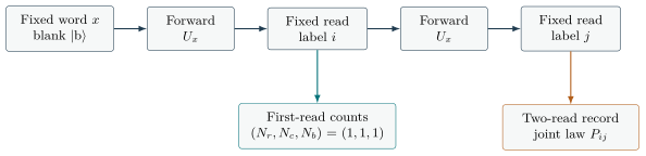
An operational statement of sufficiency must name the experiment. The wider record framework admits a typed alphabet comprising six oriented transfers, a fixed-instrument read, branch-conditioned correction, native export and the complete service instrument. “Typed” means that an operation has a specified input and output domain; a composition is allowed only when these domains match. The concrete experiment analysed here uses a much smaller part of that alphabet: prepare one fixed system word and a blank apparatus, apply a chosen completion, read the fixed pointer, retain the outcome locally, apply the same forward completion, and read again. No intervening transfer, correction, export or reset is inserted. The local conditional state update is the rank-one projective update defined below. Our positive and negative sufficiency statements refer to these specified controls.

In words, discarding the history while keeping its ledger must lose no information relevant to the permitted future questions. One unequal pair of conditional probabilities disproves this property. By contrast, showing that two different laws fit the same initial specification tests whether the law is selected; it does not by itself test sufficiency within either law. We will give both kinds of example and keep their quantifiers separate.

The general distinction is well established. Pollock and colleagues formulate multi-time quantum experiments through the process tensor, which associates probabilities with sequences of interventions [3]. Their operational Markov criterion addresses which past influences remain detectable after suitable interventions [4]. Taranto and colleagues show why quantum memory must also be discussed relative to the instruments used to probe it [5]. These references motivate our explicit control restrictions. We do not infer a process-tensor non-Markovianity theorem from a count-only counterexample. In fact, under the isolated apparatus read used here, the current label is a sufficient state for repeated uses of a fixed law.

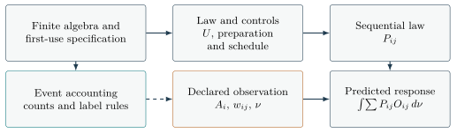
The contribution is an exact, reproducible separation of law nonselection, count insufficiency and observation dependence in this finite model. We give the complete unitary extension family, distinct worked witnesses for the first two questions, and classifications of two observation families. An exact example shows how correlations survive complete cancellation of the marginal contrast. Figure 3 summarises the dependencies between accounting and prediction. These results identify the extra inputs needed to turn record accounting into physical prediction. They neither reconstruct quantum theory nor infer a Hamiltonian, clock or coupling from an event count.

2 The finite apparatus and its disclosed premises

2.1 Words, records and the first-use map

Start with eight bits in the ordered positions $(g_0,g_1,\ell_q,c_0,c_1,i_3,\chi,w_k)$, with addresses $0,\ldots,7$ respectively. A word is valid precisely when

Thus the first pair cannot both equal one, the final pair must agree, and $\ell_q$ records whether at least one of $c_0,c_1$ is one. The bit $i_3$ is unrestricted. There are $3\times4\times2\times2=48$ valid words. The inherited names label binary positions here; no physical interpretation of those names is required for the calculation.

Let $\mathcal H_S$ have these 48 valid words as its orthonormal basis $\lvert x\rangle$. Writing the ordered bits as $b_0,\ldots,b_7$, the identifier $x$ is their binary value with the first listed bit most significant: $x=\sum_{a=0}^7 2^{7-a}b_a$. Address $a$ is active when flipping that bit changes a valid word into an invalid one. Define $A_x$ as its active address set and $n_x=|A_x|$. Enumerating the validity rule gives 4, 16, 20 and 8 words with respectively 3, 4, 5 and 6 active addresses. The accompanying verifier reconstructs this census and the entire list from Eq. (2). The word numbers are therefore not consecutive; for example, $A_0=\{2,3,4,6,7\}$ and $A_{64}=\{0,2,3,4,6,7\}$.

The apparatus space $\mathcal H_E$ has dimension ten, with basis

Here $\mathrm{b}$ means blank, $\mathrm{d}$ means idle, and $0,\ldots,7$ are numbered records. Idle is an outcome distinct from blank. Returned blank on reuse is also an outcome; calling it a reset or erasure would add an operation that is absent from our experiment. The full system–apparatus space has dimension $48\times10=480$.

Define the uniform active vector and the prescribed first-use state by

The first-use isometry sends $\lvert x\rangle\lvert \mathrm{b}\rangle$ to $\lvert x\rangle\lvert v_x(\gamma)\rangle$. The allowed interval makes every square root real for every word, and the two squared coefficients sum to one. The associated first-read probabilities are Thus the map specifies a probability per active address and a residual idle probability. It tells us what happens to a blank input; it does not yet tell us what happens when a used apparatus is submitted again.

The algebra underlying the word list and first-use instrument is documented in the frozen source collection [6]. For the theorems here, the listed active sets and Eq. (5) are the finite input data. Their microscopic geometric origin is not needed. None of the diagrams in this paper represents a spatial tiling or an identification of degrees of freedom belonging to different cells.

2.2 A read is an instrument, not just a list of probabilities

The apparatus read has outcome projectors $\Pi_i=\lvert i\rangle\!\langle i\rvert$, with $i$ running over the ten labels. On the isolated apparatus its operation is

The unnormalised operation carries both the probability of the outcome and its subsequent state. Since $\sum_i\Pi_i=I_E$, summing the outcome probabilities gives one. On the joint carrier, the read uses $I_S\otimes\Pi_i$. The system word remains fixed for our controlled completions, so the ten-dimensional calculation suffices for this experiment.

This is standard finite-dimensional quantum-instrument mathematics. Watrous [7], especially the treatment of channels, measurements and their representations, provides the general background. Stinespring’s dilation theorem [8] places isometric representations of completely positive maps in their wider mathematical setting. Our $U(432)$ freedom below follows from elementary finite-dimensional unitary extension, not from a new dilation theorem.

2.3 What is assumed, declared and derived

Terminology. A read is one invocation of the fixed measurement. A commit is a counted record change, and a bill is the service-event tally assigned to it, without an assigned monetary or energy value. Blank ($\mathrm{b}$), idle ($\mathrm{d}$) and the eight numbered records are distinct pointer labels. V1 names the declared address-transfer rule; V2 names the declared pointer-change counting rule. An identifier such as INT99 denotes a numbered audit record, not a physical quantity. These identifiers and their source history are collected in Appendix B.

The ambient framework assumes complex Hilbert spaces, an isometric record map and local tomography. An operational reconstruction such as that of Chiribella, D’Ariano and Perinotti [9] shows the kind of additional principles required if quantum theory itself is the conclusion sought. Here Hilbert-space quantum mechanics is the starting language. The explicit witnesses even use real matrices; local tomography is not needed for their calculation. No derivation of these ambient assumptions from a ledger is claimed.

Two further declarations enter the interpretation of histories. They are premises, even though their consistency has been audited. The first, called V1 in the source record, adds an address-relabel transfer production to the history grammar. It transports an occupied carrier with its internal record unchanged. That production supplies an operation; it does not supply its occurrence probability or elapsed time. Our local witness uses no such transfer, but conclusions about the wider framework remain conditional on this declared operation.

The second, V2, specifies local retention and pointer-change service counting on reuse. Every invocation is one read. A commit and one service bill are counted precisely when the new label differs from the preceding label. With the previous label $i$ and new label $j$, the increments are

These are counts, not bill values, physical energies or durations. V2 supersedes an unconditional occupied-use count rule. The source census contains 9,600 two-read history cells, of which 3,696 have positive probability at $\gamma=1/12$. Of these, 544 repeat a label and 3,152 change it. The repeat histories expose the need to distinguish an invocation from a new pointer increment. They do not establish that two histories with the same current label have different futures. At first use, blank has zero output support by Eq. (6), so every supported first outcome has counts $(1,1,1)$ under V2.

Exact accounting remains useful. The earlier audit establishes a type-preserving correspondence between the specified transfer histories and their record/commit descriptions, together with one-commit conservation on its admitted history domain. It leaves the passage from that history space to a normalised ensemble measure open. The transfer declaration is consistent on its tested source domain. These are positive results about what events mean and how they are counted, rather than a probability law for their sequence [6]. Likewise, earlier real, virtual and Coulomb classifications retain their declared dating conditions; they do not provide a clock through a change of vocabulary.

For clarity, the theorem statements below are derived mathematics on disclosed inputs. The physical choice of a completion or an observation remains open. V1 and V2 remain declarations. A source audit that reports an unselected input means unselected by a stated frozen source set; it is not an assertion that no possible theory could supply it.

3 The first-use map leaves a large reuse freedom

Write $B=\mathcal H_S\otimes\operatorname{span}\{\lvert \mathrm{b}\rangle\}$ for the 48-dimensional blank-input subspace. A completion is a unitary on the 480-dimensional carrier whose action on $B$ is the prescribed isometry. Call the class of all such completions $\mathcal E_0$. It is useful to distinguish this full class from the two examples we will calculate.

The formula means that knowing 48 input columns of a unitary leaves an arbitrary unitary action on their input complement. It is not a count of 432 alternative laws: $U(432)$ is a continuous group. Nor does the formula assert that every member preserves the system word. Our two witnesses do, while the full extension class also permits mixing consistent with the fixed blank columns. Extra symmetries or locality constraints could reduce this family, but must be supplied with their proper domains.

There is also a simple obstruction to retaining the entire first-read supported space on reuse. For $0<\gamma<1/6$, define

Its dimension is $48+\sum_x n_x=48+224=272$. The spaces $B$ and $R$ are orthogonal, and $UB\subset R$ for every admitted completion.

Some occupied directions must therefore leave $R$. This is a rank statement, not a lower bound on a leakage probability for an arbitrary input. It does not say that every used input leaves $R$, or that an output outside $R$ is erased. It shows why a rule written only for first-use supported records cannot automatically serve as a closed rule for reuse.

4 Two laws, and a separate witness within one law

4.1 Two explicit completions

Fix a word $x$, abbreviate $n=n_x$ and $t=1-n\gamma$, and define

The vectors $\lvert \mathrm{b}\rangle,\lvert v\rangle,\lvert w\rangle$ are orthonormal. On $\mathcal H_E$, set The first operator interchanges blank and $v$ and fixes their orthogonal complement; the second cycles blank to $v$, $v$ to $w$, and $w$ to blank, fixing the remaining directions. Hence $H_x^2=I_E$ and $C_x^3=I_E$. Both are unitary and both send blank to $v$. Their controlled direct sums over $x$ belong to $\mathcal E_0$, and either can be used as $U_0$ in Theorem 3.1.

The sign of $w$ matters for the cycle and is fixed by Eq. (12). An alternative formula in the sources, $(\lvert \mathrm{d}\rangle-\sqrt t\lvert v\rangle)/\sqrt{n\gamma}$, is identical for $\gamma>0$. The accompanying verifier checks that equality. Invertibility does not choose between these examples: $C_x^{-1}=C_x^\dagger=C_x^2$, but another forward application of $C_x$ is not its inverse. Replacing the second invocation with an adjoint would change the experiment.

After the first projective read returns $i$, the local state is $\lvert i\rangle$. The ordered two-read joint law is therefore

The first factor is the chance of reaching $i$; the second is the conditional chance of reaching $j$ from there. Rows index the first read, columns the second. Summing rows or columns yields the appropriate marginal, while retaining the table keeps their correlations.

4.2 The first-use specification does not select the future law

All numerical results from here on use the declared test value $\gamma=1/12$. This value supplies an exact discrimination experiment; it is not inferred as a physical constant. There are 96 processes: both laws on each of 48 preparations. At word 0, summing the second-read probabilities into blank, idle and all numbered records gives Table 1.

The different blank probabilities already separate the laws using the existing fixed read. Both laws obey exactly the same first-use isometry, not merely the same first histogram. Thus even full knowledge of that isometry cannot select the future law. The second-read marginals differ on 40 of the 48 words. On the other eight they coincide, but the joint tables still differ, as Section 6 shows.

4.3 The count ledger is insufficient after the law is fixed

Now choose $H$ alone. At word 0, the first idle outcome has probability $7/12$; each of the five active numbered outcomes has probability $1/12$. Every one of these events has first-use ledger $(1,1,1)$, yet

These are two reachable histories with equal counts, one fixed law, the same future operation, and unequal conditional futures. They disprove Eq. (1) for the count-only ledger. No comparison between different laws is needed. Under $C$ the analogous conditionals are $5/12$ after idle and $7/60$ after each active numbered outcome, so the same count-only failure occurs there as well.

The two histories have different current labels. This is precisely the information the count ledger omitted, and it limits the conclusion. We have not proved insufficiency for a ledger that also retains the label. Indeed, the opposite statement holds on this isolated apparatus.

In particular, repeating a label does not leave distinguishable local history behind in this rank-one model. Under repeated fixed reads its labels form a Markov chain with transition probabilities $T^U_{ji}=|\langle j|U_x|i\rangle|^2$. Count insufficiency here is a coarse-graining failure and can occur in an ordinary classical description of this chain. Classical lumpability studies which probabilities are preserved exactly when states of a Markov chain are aggregated; see Buchholz [10]. Our criterion retains questions about future record labels, not merely whether the count process itself is Markovian. The witness is not evidence of specifically quantum memory beyond the current label.

On the full 480-dimensional carrier, $I_S\otimes\Pi_i$ instead has rank 48. A read can leave different conditional system states associated with the same apparatus label. This observation locates where a richer memory question would have to be tested; it does not produce a reachable witness. The 544 supported repeat-label histories are therefore not a substitute for such a test.

5 What a three-parameter observation retains

5.1 A declared family of stochastic responses

An apparatus record and an observed response need not have the same alphabet. The earlier carrier-map audit left both the physical map type and the relevant input/output actions unselected [6]. For example, a stochastic map from ten labels to four response outcomes is different from ten matrices acting on a four-component mode. These types require different compatibility equations. A type signature organises the question; it does not choose an operator or identify a physical response.

Nevertheless, a declared mathematical family can be classified without pretending it has been selected by the framework. The first family, $\mathcal K$, is the authenticated symmetry fixture used in the source audit. Its covariance constraints have rank 37 on the 40 matrix entries. The action has six entry orbits of sizes $1,3,1,3,8,24$; column normalisation leaves three parameters. Nonnegativity gives exactly

The fixture uses a declared group action of order 48 and has eight extreme points, the cube vertices. These are facts about that action and that stochastic type, not a classification of all physically admissible bridges.

Each column $M_i$ is a probability distribution over four response outcomes. Its distinguished response has probability $a$, $b$ or $c$ according to whether the record was blank, idle or numbered. All eight numbered records have the same response column. The map discards their individual identities before any further statistic is computed.

For a second-read marginal $p$, define $f(p)=(p_{\mathrm{b}},p_{\mathrm{d}},p_{\mathrm{N}})^T$, where $p_{\mathrm{N}}=\sum_{j=0}^7p_j$. The response marginal is

This formula says exactly what the observation retains: three population totals. For any declared set of inputs, two parameter triples give the same responses precisely when their difference is orthogonal to the span of its feature vectors $f(p)$. In the full set of 96 test processes this span has rank three: the rows from $(0,H)$, $(0,C)$ and $(40,H)$ have determinant $-5/5184$. Consequently distinct parameter triples can be distinguished by some input in that set. This does not mean that every fixed triple distinguishes all processes.

5.2 Marginal blindness and its exact range

Let $\Delta$ denote $H-C$ at the same preparation. The exact tables give

For $n=3,4,5$, the marginal contrast vanishes on a plane in the parameter cube. For $n=6$, every point in the cube hides the marginal contrast. Across all preparations the contrast vectors span a two-dimensional space, so the maps invisible to all these $H/C$ marginal comparisons are exactly $a=b=c$.

At word 0 the formula reduces to

Equality of the blank and numbered columns is not enough to hide this contrast: $(a,b,c)=(0,1,0)$ gives $-5/144$. Conversely, a nonconstant map can hide it: $(5/12,1,0)$ gives zero. A particular cancellation is different from structural loss of a whole label distinction.

The total-variation distance between two response distributions is half the sum of the absolute component differences. Here those differences are $(\delta,-\delta/3,-\delta/3,-\delta/3)$, so

Write $\bar t=(n/12)b+(1-n/12)c$. Since $\bar t\in[0,1]$ and $a\in[0,1]$, $\Delta q_0=d_n(a-\bar t)$ gives $|\Delta q_0|\leq d_n$. For $n<6$, equality is attained at $(1,0,0)$; for $n=6$ the distance is zero everywhere. The minimum is attained at any invisible map. Intermediate values follow by continuity. Thus these ranges hold without choosing a preferred map.

5.3 The same map can also be used in a two-read observation

It would be incorrect to call $\mathcal K$ intrinsically a single-read observation. Apply its response independently to both slots of the joint table and ask for agreement of the two response outcomes. This gives

where $R$ is the joint table after grouping labels into blank, idle and numbered, and $(t_{\mathrm{b}},t_{\mathrm{d}},t_{\mathrm{N}})=(a,b,c)$. The dot product is the agreement probability for two independent response draws, conditional on the respective records. This response randomisation is part of the declared observation; the record table itself need not factorise.

Since $k(s)^Tk(t)=(1-s-t+4st)/3$, the $H/C$ contrast is a quadratic polynomial in the three parameters. Its exact ranges are shown beside the marginal ranges in Table 2. They are obtained from stationary points on every cube face, with the singular cases reduced to their boundaries, not merely by sampling the vertices. Appendix A gives the polynomials and the completeness argument.

For $n<6$, the lower endpoint of the signed range is attained at $(0,1,1)$ and the upper at $(1,1,0)$. For $n=6$, the contrast is identically zero, so no response is distinguished as a unique optimiser. Equal columns within each group retain the joint table of the groups; they do not reduce it to one marginal. Equal columns across all labels instead give $F=\|M_i\|^2$ for every normalised $P$, which is process independent under the unit weighting used here.

6 Label-sensitive observations and the six-label cancellation

6.1 A second, explicitly different mathematical type

The second family, $\mathcal T$, consists of ten nonnegative column-stochastic $4\times4$ matrices $A_i$, one for each apparatus label. It has 120 free coordinates: each of the 40 columns is a four-component probability vector, subject to one normalisation. Let

The vector $r$ is an input mode, not an apparatus record and not an extra system preparation. Its interpretation is part of the declared test observation. Each $m_i(r)$ is again a probability distribution. The unweighted two-slot agreement functional is The tensor notation packages how the record, input mode and output response meet. It does not add a physical rule assigning any of those roles. In particular, covariance of $\mathcal K$ cannot be borrowed for $\mathcal T$: transformations of the labels, mode inputs and response outputs, and the way the tensor transforms, must be specified first.

The embedding $A_i=M_i\mathbf1^T$ realises $\mathcal K$ inside $\mathcal T$: all four columns of $A_i$ equal $M_i$, hence $A_i r=M_i$ for every normalised $r$. Thus $\mathcal T$ contains the simpler two-slot observations, while also permitting different responses for different numbered records. This is a mathematical inclusion of test families, not a physical choice between their interpretations.

6.2 Which tensors and which processes are observationally equivalent?

Only the symmetric part of $Q$ contributes to $r^TQr$; an antisymmetric matrix has zero quadratic form. Over the full mode simplex, two responses $A$ and $B$ agree for every admitted process $P$ if and only if

There is a finite identifying test: a symmetric $4\times4$ matrix $D$ is determined by its quadratic form on the four vertices and six edge midpoints of $\Delta_3$. Specifically, The mode values first recover the four diagonal entries and then the six cross terms. This is an observation-equivalence test, not proof that the ten modes can be prepared in a physical implementation. On a restricted mode set one obtains only equality of the corresponding quadratic values, equivalently equality on the span of the admitted matrices $rr^T$.

There is a complementary question: hold the entire observation family available and ask which process tables it can distinguish.

The quotient belongs to this specified unweighted family. It is not the information content of an unrestricted two-read record: directly observing an ordered event can distinguish an antisymmetric change in $P$. Nor does the result say that all possible normalised pair tables are reachable. Those tables provide a mathematical comparison domain in the proof; the operational denominator remains 96.

6.3 An exact cancellation with a visible correlation

At each of the eight preparations with $n=6$, the second-read populations are identical under both laws:

The value $3/32$ is for each of the six active numbered labels; the two inactive labels have zero probability. The first marginals also agree because the first-use map agrees. Consequently no function of either individual-read distribution can separate these laws here, even if it retains every numbered label.

The reason can be proved without a small-difference approximation. At $n\gamma=1/2$, the frozen vectors are $v=(\lvert \mathrm{d}\rangle+\lvert u_x\rangle)/\sqrt2$ and $w=(\lvert \mathrm{d}\rangle-\lvert u_x\rangle)/\sqrt2$. The second vector is antisymmetric between idle and the active collective vector. Direct substitution into Eq. (15) yields the following identity.

The positive diagonal change is compensated by five equal negative off-diagonal changes in each row. Summing over either read therefore removes the difference exactly. Summing all active labels into the numbered group removes the whole block as well. Thus $\mathcal K$ discards distinctions within each label group, and at $n=6$ the $H/C$ joint-table difference vanishes entirely under that grouping. This is stronger than marginal equality, and explains the zero in the last row of both range columns in Table 2.

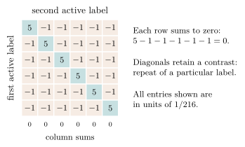
Fix one active label $i$, for example numbered label 0 at word 64. Assign it the response $e_0$ and every other record the response $e_1$, using constant columns in every $A_i$. These two responses are orthonormal unit vectors, so their dot product is one for agreement and zero for disagreement. The functional therefore asks whether both reads agree on the binary question “label $i$ or something else”. For this choice it is

The joint repeat probabilities are $P^H_{ii}=121/1728$ and $P^C_{ii}=3/64$, differing by $5/216$. These are joint probabilities, not conditionals. Dividing by the common first probability $1/12$ gives conditional repeats $121/144$ and $9/16$. The first value also appears as the exact maximum in the earlier pointer-count audit.

Three quantities must not be conflated. The joint repeat contrast for one active label is $5/216$. Binary agreement has contrast $5/108$, because with equal marginals the coefficient of $P_{ii}$ in Eq. (34) is two. The event “the second read repeats whichever active numbered label came first” sums all six diagonals and has contrast $5/36$. Each is a legitimate question, but they are different observations.

Furthermore, $5/108$ is a certified witness, not an upper bound on $\mathcal T$. Equation (33) gives the direct corollary

To see this, expand the squared differences: each squared norm appears five times and every cross term twice, exactly reproducing the diagonal and off-diagonal coefficients of the block. Assigning three active labels to $e_0$ and three to $e_1$ gives nine nonzero differences of squared length two, hence $\Delta F=1/12$. This exceeds $5/108$. The identity and this example are explanatory corollaries of the frozen tables; neither asserts the solution of the full 120-coordinate optimisation.

7 Weights and measures are part of the observation

7.1 Effective pair responses

The preceding ranges use normalised joint tables and unit weights. If a service rule assigns a pair weight $w_{ij}$, the observed contraction instead uses

On an admitted process family, invariance means exactly that $O$ is orthogonal to every difference $P-P'$ in that family. If the comparison domain is the full simplex of pair tables on a specified support, this holds if and only if $O$ is constant on that support. Delta tables prove necessity, and normalisation proves sufficiency. This elementary pairing criterion is the appropriate way to restate an invariance theorem after weights have been introduced.

For factorised service weights $w_{ij}=s_i s_j$, one can equivalently use effective responses $\widetilde m_i=s_i m_i$. Equality of all effective responses is sufficient for process independence. General pair weights cannot be absorbed this way. Under V2’s label-change predicate $w_{ij}=\mathbf1[i\ne j]$, equal unweighted responses $m_i=m$ give

The factor $1-\operatorname{tr}P$ is the probability that the label changes. It can depend on the process despite equality of every unweighted column. Weighting therefore changes the observation, rather than merely changing its notation.

These weighted quantities are generally unnormalised expectations. If one instead wishes to condition on a service event, one must divide by its probability when positive. That defines another statistic and must be declared separately. Likewise, replacing $P_{ij}$ by $p_i^{(1)}p_j^{(2)}$ assumes independence between reads. It discards the very correlation measured in Section 6. Neither replacement follows from agreement of event counts.

7.2 Averaging over modes

For a declared probability measure $\nu$ on the mode simplex, define its second-moment matrix $\Sigma_\nu=\int rr^T\,d\nu(r)$. Then

This is simply the integrated quadratic form written as a matrix contraction. It exposes the precise measure information needed: for this functional only the second moments matter. Equality for one measure is one contraction condition; equality for every probability measure implies pointwise equality, since point masses at individual modes are included.

For fixed $A,P$, continuity on the compact simplex gives a minimum and maximum of $F$. Every probability integral lies between the minimum and maximum of $F$. Point masses at minimising and maximising modes attain the endpoints, and their mixtures fill the interval. This is a mathematical statement about the class of all measures, not a claim that any such measure is physically available.

A simple example separates process independence from measure independence. Take $A_i=I_4$ for every label and unit weights. Then

The minimum is at the uniform mode and the maximum at a vertex. The process has disappeared, but the mode and its measure have not. For the historical test normalisation the corresponding all-measure range is $[1,11/8]$. The affine slope also explains why the binary witness contrast $5/108$ in $F$ becomes $5/216$ in $K_{\rm test}$ when the same measure and unit weights are used.

The historical kernel calculation averages four monitored direction weights over a uniform four-torus, with $r_\mu=\sin^2(k_\mu/2)/\sum_\alpha\sin^2(k_\alpha/2)$ away from the zero-denominator set, which has measure zero. Its four direction labels are not the ten apparatus records of this paper. Their identification and a response map remain additional inputs. Accordingly, the present separation results make no claim that a physical endpoint coefficient called $K_2$ detects $H$ versus $C$. They show that specified label-sensitive two-slot observations can do so. The historical normalisation is retained here only to make the observation and measure distinction explicit [6].

8 What must be supplied to derive physics

The examples expose three distinct levels of incompleteness. A first-use isometry can leave the future law unselected. A fixed law can act on states that a count ledger fails to distinguish. Even a completely known pair table can yield different measured responses when the observation map, weights or sampling measure change. Fixing one level does not fix the others. Figure 3 makes these dependencies explicit.

The wider source audit also leaves the schedule, clock assignment and absolute normalisation unresolved. Appendix B gives the detailed inventory and source identifiers in Table 3. These obligations may constrain one another in a future theory; they are not a count of independent numerical parameters. A physical law may be added, but its introduction is a further premise rather than a consequence of the ledger alone.

The absolute-unit issue deserves particular care. It is not the familiar freedom to express a length in metres or centimetres. The earlier audit finds an unselected dimensionless normalisation needed to identify two proposed accounting units; alternative interpretations preserve the admitted algebraic observations [1]. No value for it is inferred from the response examples in this paper.

A sufficient predictive description can be given without claiming it is minimal. Specify the joint system–apparatus state, the law, the admissible instruments and their scheduling rule. Iterating those instruments gives the future probabilities. If a smaller description is desired, its sufficiency is a theorem about the chosen law and controls. The count-only counterexample rules out one compression. Proposition 4.1 validates another compression on the isolated apparatus. Neither decides the minimal predictive state of the coupled framework.

The finite observation quotient suggests a restrained order for further work. First identify the distinctions an intended experiment can observe. Then specify only the remaining physically relevant freedom needed to predict them, and state any unobservable freedom as an equivalence class. This avoids demanding a unique matrix representation when a family of representations has the same operational content. Conversely, quotienting by a chosen observation does not justify discarding distinctions that a different, physically admitted observation would retain.

There are concrete next questions. To test a label-retaining ledger on the joint carrier, hold the law fixed and search for two reachable histories with the same ledger and current apparatus label but different future read probabilities. A null result on the isolated ten-dimensional apparatus cannot settle that question. To identify a physical response, one must state how actual record labels become the monitored quantities, and then calibrate or derive its columns, weights and measure. Process tomography is relevant only over the linear span of instruments that can actually be implemented; the present operation alphabet has not been proved tomographically complete.

Composition of successive observations and stability under refinement of record descriptions are possible additional consistency requirements. They are questions for a further specified study, not assumptions inserted into the present calculation. The completed audit selected no physical bridge. A new physical selection claim requires its own explicit premises and evidence.

9 Reproducibility and the strength of the evidence

The principal source is the closed audit of the two observation families, with its inputs fixed by a source manifest [6, 11]. The two original routes reproduce earlier exact joint tables, and an independent review reconstructs the results from those tables. Controls and deliberately perturbed inputs test both the calculation and rejection of unsupported scope changes. Appendix B records the source identifiers and verification counts; these describe audit coverage, not probabilities that the theory is true.

The two original computational routes use different exact constructions. Route A constructs amplitudes and symbolic contractions with SymPy. Route B uses rational quadratic-field arithmetic and a separate transition-block construction. They share authenticated inputs and a report schema but do not import one another’s operative solver. Both reproduce the exact earlier INT96 tables and produce the same scientific certificate. Some individual $C$ entries for $n\ne6$ contain square roots; the stored pairs encode $u+v\sqrt d$, not real and imaginary parts or rounded decimals. The rational population totals result from exact sums.

The portable supplement accompanying this paper contains the 48 active-set profiles, all 96 exact two-read tables, the relevant certified observation data, a manifest binding them to git blobs by SHA-256, and verify_paper.py. That verifier reconstructs $H$ and $C$ directly from Eqs. (13)–(14), checks the joint laws and marginals, recomputes the ranks, exact face extrema and finite symmetric quotient, and checks the six-label block and response-distance corollary. It also verifies the count witness, support census and rank-one identity. It is a paper-level regression and proof aid, not a new governed result bank or a replacement for the original independent routes.

The analytic proofs establish the universal parts of the claims: unitary extension, the rank bound, sufficiency of a rank-one current label, the observation-equivalence criteria and completeness of the extrema search. The exhaustive finite tables establish the stated census and distinguish the particular processes. Source-review controls test that unsupported scope changes are rejected; they do not prove that every rejected extension is mathematically false. Likewise, agreement of two programs supports the implemented calculation but cannot replace checking that its inputs represent the intended experiment.

There are deliberate limits. This paper does not optimise $\mathcal T$ over all 120 free coordinates, classify the full $\mathcal E_0$ family up to every possible experiment, or search for joint-carrier label-memory witnesses. It contains no fit to experimental constants. Its physical nonselection statements are relative to the audited source sets; its finite counterexamples are explicit mathematical statements with the conditions printed in the text.

10 Discussion and conclusion

The strongest objection to the headline is that a ledger was never promised to contain a dynamical state. If it is intended only as an event counter, count insufficiency is expected and does not undermine its accounting role. The objection is correct. The significance arises when exact counting identities are used to support a stronger inference: that the framework already determines sequential probabilities or a downstream physical response. The explicit counterexamples show where that inference needs additional premises.

The result also does not identify an inconsistency in quantum mechanics. Both $H$ and $C$ are ordinary unitary completions of the same isometry. Their existence is a concrete expression of extension freedom. The count-only failure is visible in a classical stochastic description after the fixed rank-one read. Claims about specifically quantum memory on the larger carrier therefore remain separate from the conclusions established here.

What is less immediate, and useful for the framework, is the exact dependence on the observation. At six active addresses the complete single-read distributions agree, yet the ordered records retain a nonzero difference. A map that identifies all numbered labels removes that difference even in a two-slot statistic. A label-sensitive response can retain it. The explicit block identity explains the cancellation and the exact ranges quantify what survives in the declared simpler family. The 24-class quotient then states exactly how much of the finite process set the richer, unweighted Gram family identifies.

The resulting conclusion is constructive. Identical single-read statistics can conceal different sequential laws. Their distinguishability depends on which joint record distinctions the observation retains; specifying its mathematical type is necessary, but its response map, weights and measure must also be supplied. The ledger fixes a disciplined account of events. A predictive physical theory must additionally explain the law of their succession and the observation through which that law is tested.

Declarations

Data and code availability. The accompanying source package includes the manuscript, bibliography, TikZ diagrams, exact fixture data, source manifest and portable verifier. The preprint and portable source package are deposited at doi:10.5281/zenodo.22541078. The historical audit sources are identified by immutable repository commits in Appendix B and reproduced in the frozen companion archive, doi:10.5281/zenodo.22541080. Both the selected audit collection and its INT99 dossier component are cited at this archive DOI. Compilation requires a standard TeX distribution; verification requires Python 3 and SymPy. No proprietary numerical solver or network access is needed to run the supplied verifier.

AI assistance. OpenAI Codex assisted with source inspection, exact-computation orchestration, reference checking, LaTeX drafting and layout verification. AI-generated prose is not an independent source of evidence. The mathematical claims are supported by the disclosed definitions, proofs, source records and executable checks; responsibility for the submitted manuscript rests with the author.

Affiliation and interests. The author is affiliated with Neuro-Symbolic Ltd, which is associated with the framework discussed here. This affiliation is disclosed for readers assessing the work.

A Closed formulas and exact range certificates

Summing Eq. (15) gives, for general $n$ at $\gamma=1/12$,

The numbered total is one minus the other two components. These formulas produce Eq. (22); the verifier also obtains them by direct matrix contraction. The $\mathcal K$ two-slot contrast polynomials are The extra factors show why a two-slot contrast can have zeros beyond the corresponding marginal-invisibility plane. Equality for one statistic is not equality of the grouped joint table.

For completeness, a quadratic on the compact cube attains its extrema. Each extremum lies in the relative interior of a face, where its gradient in every free coordinate vanishes. There are $3^3=27$ faces when each coordinate is designated free, fixed at zero, or fixed at one. On each face, solve the linear stationary system and retain the solutions inside that face. If the restricted Hessian is singular and a stationary point exists, a nonzero null direction of that restricted Hessian leaves the quadratic constant. Moving along it reaches a boundary face with the same value. Repeating reaches a face with a nonsingular stationary system or a vertex. Thus nonsingular feasible stationary points together with vertices suffice. This proves the completeness of the finite search used for Table 2.

The ten-mode reconstruction in Eq. (29) can also be checked as a matrix inversion. Its evaluation determinant is $1/64$ in the basis $(r_\mu^2,2r_\mu r_\nu)$ and $1/4096$ in the monomial basis $(r_\mu^2,r_\mu r_\nu)$. Invertibility is the invariant claim; the determinant’s numerical value depends on the coefficient convention.

B Source status and provenance

The manuscript structure follows the note “The Ledger Is Not Enough: paper structure” at commit c8cb7e63; its exact path and hash are listed in the accompanying source manifest. Its earlier prospective wording is updated to the closed INT99 result bank. The subsequent DRIFT propagation at 0a8f7cb6 records that terminal result without changing its scientific status. Neither presentation commit supplies a new physical premise. The latest governed count is 255, with $\binom{255}{2}=32{,}385$ pairs; this is audit bookkeeping, unrelated to an experimental probability.

In these records, “banked” means committed after the project’s prescribed independent countersign; it does not mean peer reviewed by a journal. The INT99 source manifest contains 167 units. Its dossier records 32 controls and 16 seeded probes over eight mechanisms, and 23,955 checks in the bundled verifier. These are coverage and provenance counts, not weights of scientific evidence. The audit granted no successor licence.

The INT99 parent ruling was banked at 730ef689. Its result dossier is closed, with scientific certificate identifier

It retains two owner declarations and does not promote $H$, $C$, a map, a service weight, a measure or an endpoint to a physical selection. The new block and distance explanations in Section 6 are checked paper corollaries of its tables, not edits to the sealed certificate. Original source documents sometimes retain construction-time phrases such as “prepared for countersign”; the bank commit and countersign record, rather than those historical headers, fix their present status.

The wider input inventory in Table 3 also draws on the normalisation audits INT81/81P and the clock, dating and schedule audits INT90 and INT93–95. Their use here is limited to their recorded selection boundaries. We do not transplant an earlier continuum or geometric calculation into the finite apparatus model, or infer a new physical observable from a similarity of numerical expressions.

References

1. David G. Elliman. Described twice? A finite audit of a possible gravity–measurement seam. Zenodo preprint, version 0.5, 2026. doi:10.5281/zenodo.22407952.
2. David Elliman. Pointer states are not enough: Physical monitor selection in a finite quantum register. Zenodo technical note, version 1.0, 2026. doi:10.5281/zenodo.22003393.
3. Felix A. Pollock, César Rodríguez-Rosario, Thomas Frauenheim, Mauro Paternostro, and Kavan Modi. Non-Markovian quantum processes: Complete framework and efficient characterization. Physical Review A, 97: 012127, 2018. doi:10.1103/PhysRevA.97.012127. arXiv:1512.00589.
4. Felix A. Pollock, César Rodríguez-Rosario, Thomas Frauenheim, Mauro Paternostro, and Kavan Modi. Operational Markov condition for quantum processes. Physical Review Letters, 120: 040405, 2018. doi:10.1103/PhysRevLett.120.040405. arXiv:1801.09811.
5. Philip Taranto, Felix A. Pollock, Simon Milz, Marco Tomamichel, and Kavan Modi. Quantum Markov order. Physical Review Letters, 122: 140401, 2019. doi:10.1103/PhysRevLett.122.140401. arXiv:1805.11341.
6. David G. Elliman. The ledger is not enough: Frozen audit sources and INT99 result dossier. Zenodo dataset, version 1.0, 2026. doi:10.5281/zenodo.22541080.
7. John Watrous. The Theory of Quantum Information. Cambridge University Press, Cambridge, 2018. doi:10.1017/9781316848142.
8. W. Forrest Stinespring. Positive functions on $C^*$-algebras. Proceedings of the American Mathematical Society, 6 (2): 211–216, 1955. doi:10.1090/S0002-9939-1955-0069403-4.
9. Giulio Chiribella, Giacomo Mauro D’Ariano, and Paolo Perinotti. Informational derivation of quantum theory. Physical Review A, 84: 012311, 2011. doi:10.1103/PhysRevA.84.012311. arXiv:1011.6451.
10. Peter Buchholz. Exact and ordinary lumpability in finite Markov chains. Journal of Applied Probability, 31 (1): 59–75, 1994. doi:10.2307/3215235.
11. David G. Elliman. Typed carrier-map observables: INT99 result dossier. Eight-artifact component of the frozen audit archive, version 1.0, commit 13eb46ca, 2026. CANON, exact routes, comparator and freeze; doi:10.5281/zenodo.22541080.