The Holographic Quantum Stack Machine (HQSM) is a finite quantum architecture in which distributed registers carry internal degrees of freedom and pairs of boundary addresses define an interior spatial representation. We give a mathematical specification of an eight-site prototype and distinguish its exact properties from its proposed interpretation in particle physics. Explicit [[8,2,2]]₂ and [[8,2,2]]₃ stabilizer encodings hide logical information from any single ledger site. A 64-dimensional chord register contains an isometric 32-dimensional shell–anchor representation with an exactly computable radial hopping operator. Integer registers provide reversible bookkeeping for selected quantum numbers. We replace an unrestricted pair of controlled-NOT gates by a chirality-selected exchange that conserves electric charge on the entire state space, and describe auxiliary-sector elimination using the Schur complement. A three-component mass ansatz reproduces the Koide identity only on the appropriate positive-root branch; its proposed fixed phase is incompatible with the precision muon–electron mass ratio. An explicitly calibrated version gives a testable, conditional tau-mass estimate. Positive boundary weights yield a bounded barycentric map, but do not supply a spacetime metric or gravitational field equations. Reproducible calculations separate these finite algebraic results from the additional dynamics, symmetries and continuum limits required for a physical theory. The construction is presented as a computational model and research framework, with derivations accessible to readers familiar with undergraduate linear algebra and quantum mechanics.
Elliman, D. (2026). The Holographic Quantum Stack Machine: A finite boundary-encoded architecture for particle-like states. Neuro-Symbolic Ltd technical report. https://doi.org/10.5281/zenodo.23991267
@techreport{elliman2026holographicquantumstackmachine,
  author      = {Elliman, David},
  title       = {The Holographic Quantum Stack Machine: A finite boundary-encoded architecture for particle-like states},
  institution = {Neuro-Symbolic Ltd},
  year        = {2026},
  doi         = {10.5281/zenodo.23991267},
  url         = {https://neusym.ai/papers/holographic_quantum_stack_machine/}
}
Full text
The complete paper, rendered as HTML with the mathematics set at build time. The PDF above is the typeset version
of record; equation, theorem and reference numbers match it.
1 Introduction and scope
Computer architecture offers a useful language for separating the definition of an object, its stored state, its address and the operations acting on it. In quantum physics the corresponding separation is between a species of excitation, its Hilbert space, a spatial representation and an evolution law. The HQSM explores this analogy with explicit finite matrices. Its starting question is computational: can a small boundary register encode internal quantum information and an interior position representation, while maintaining reversible dynamics and specified conservation laws?
This question is related to quantum simulation, whose purpose is to reproduce the dynamics and measurement statistics of a quantum model [1]. It also draws inspiration from holographic descriptions and the relation between bulk reconstruction and quantum error correction [2, 3]. Those theories provide motivation rather than a derivation of the present architecture. Here, “holographic” means that an interior description is encoded in designated boundary-address and ledger registers. It does not assert an AdS/CFT duality, an entropy–area law or a theory of quantum gravity.
The identity of electrons does not require a common mutable memory location. In quantum field theory, electrons are excitations of the same field, with common couplings and fermionic statistics [4]. Likewise, sharing a class definition in software does not force different instances to share their runtime state. We therefore separate a shared classical species table from independent logical quantum degrees of freedom. A pointer selects a logical subsystem or spatial address; it does not clone an unknown quantum state [5].
The paper has three aims. First, it gives definitions and short proofs for the parts of HQSM that can be made exact: finite encodings, register operations, conservation tests and auxiliary-state elimination. Second, it provides a corrected reference implementation for two problematic extensions: the weak-interaction gate analogy and the charged-lepton mass ansatz. Third, it identifies the additional results needed to connect a finite architecture to measured particle physics. Neither an exact matrix identity nor a passing software test, by itself, establishes that the matrix describes nature.
1.1 How to read the model
We use three levels of statement throughout. A definition specifies a chosen model. A finite-model result follows from that definition and can be proved or checked. A physical hypothesis identifies a model quantity with an observable and must be tested independently. For example, a negative eigenvalue shift of a finite Hamiltonian is a result; calling its absolute value an electron mass is an additional hypothesis.
Table 1. The scope of the construction. The third column states what the finite result does not establish.
Component
Established within the specified model
Additional physical requirement
Boundary ledger
Two logical qudits protected against one known-site erasure
Scalable storage, preparation and physically local access
Chord pointers
Four exact chord-radius values and an isometric shell representation
A rotationally and relativistically consistent continuum limit
Register transactions
Reversible shifts and selected conserved quantities
Gauge dynamics, spin representations and scattering amplitudes
Auxiliary sectors
Exact stationary Schur reduction
Controlled dynamical approximation and physical mass matching
Generation ansatz
A conditional Koide relation
A mechanism fixing parameters and radiative corrections
Barycentric map
Convexity and an antipodal tanh identity
Metric, causal structure and gravitational field equations
1.2 Notation and prerequisites
A ket ∣ψ⟩ is a column vector and its adjoint ⟨ψ∣ is the conjugate row vector. A normalized pure state satisfies ⟨ψ∣ψ⟩=1. A density matrix ρ is positive and has unit trace; it represents pure or mixed states. A tensor product describes jointly available degrees of freedom. An isometryV satisfies V†V=I and preserves inner products while embedding a smaller space in a larger one. A projector P=P2=P† selects a subspace. An observable A is conserved by a time-independent Hamiltonian H when [H,A]=HA−AH=0.
Except when quoting particle masses in MeV, numerical energies and lengths in the finite prototype are in model units. We use ℏ=c=1 in dynamical equations and the +−−− metric convention when discussing four-momentum. The physical local dimension d∈{2,3} is distinct from the code distance, which is two in both constructions. A qubit has dimension two and a qutrit dimension three. The cube graph is denoted Q3; it is not a qutrit.
2 Architecture and resource accounting
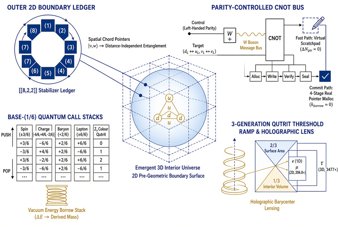
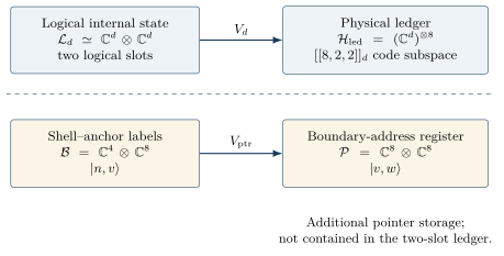
Let V={0,1}3 be the eight vertices of a cube. Vertices are connected when their binary labels differ in one coordinate. The graph has 12 edges. Adding its six square faces gives a closed cell complex homeomorphic to a two-sphere. The graph alone is a one-dimensional complex; it is the boundary cell complex that justifies the term “surface”. Figure 1 gives the motivating architectural overview; figure 2 separates the two encodings used in the formal model.
For each local dimension d define a physical ledger
Hled,d=(Cd)⊗8,Vd:Ld=(Cd)⊗2⟶Hled,d.(2.1)
The image of Vd is a stabilizer code. The qubit and qutrit ledgers may be used together, in which case the physical ledger dimension is 68 and its logical dimension is 2232=36. This counts internal storage only.
A separate pointer register is
P=span{∣v,w⟩:v,w∈V}≃C8⊗C8.(2.2)
It needs six qubits in a binary address implementation. For N labelled pointer registers the address space has dimension 64N. Allocating another pointer therefore requires additional capacity; it is not supplied by a two-logical-qudit code. A closed quantum circuit has a fixed Hilbert space, so allocation must mean activating pre-existing blank registers or moving between occupation sectors of a specified Fock space. For identical fermions, the appropriate many-particle construction is the antisymmetric Fock space over the one-particle space. Antisymmetry is an imposed kinematic structure, not a consequence of shared addressing.
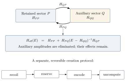
Figure 1. Conceptual overview supplied with the HQSM proposal, retained as an architectural guide. The register ring is schematic and repeats site labels; the mathematical model has exactly eight sites. “Left-handed parity” is interpreted as chirality, and the corrected operation is the charge-preserving exchange in section 6. “Borrow” denotes an auxiliary excitation cost, not a violation of energy conservation. The mass and area–volume labels describe the motivating ansatz rather than derived physical laws. The additional diagrams below specify the mathematical construction precisely.Figure 2. Two distinct encodings. The upper map distributes internal logical information over physical ledger sites. The lower map encodes shell–anchor labels into a separate boundary-address register. The registers can be combined by tensor product; neither is identified with the other.
The address v names a site but does not by itself specify where the bits representing that address are physically stored. Thus a claim that all hardware is confined to the boundary still requires a placement and routing scheme for the pointer, stack and controller registers. The present specification treats their storage as additional boundary resources. Error correction of the ledger does not automatically protect these resources.
This distinction also sets a locality requirement. If a logical operator has support on several sites, it needs a physical implementation using available couplings, gates or measurements. The absence of a bulk distance in the encoding does not make such an operation instantaneous or cost-free.
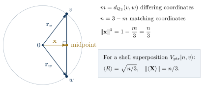
The embedding is prescribed; it is not dynamically derived. Let m=dQ3(v,w) be the Hamming distance, namely the number of differing binary coordinates, and put n=3−m.
Proposition 3.1 (Chord-radius identity). For every ordered pair (v,w),
∥x(v,w)∥2=3n,Rn=n/3∈{0,1/3,2/3,1}.(3.2)
Proof. In each of the m differing coordinates, the two signs cancel. In each of the n matching coordinates, the midpoint is ±1/3. Squaring and summing gives n/3. ◻
The 64 ordered chord labels give only 27 distinct midpoint positions, with shell populations 1,6,12,8 from the centre outward. Several different register states therefore have the same position. The finite construction does not fill a continuous ball. Its chord midpoints lie in the inscribed cube, and even arbitrary positive endpoint weights remain in that cube’s convex hull.
Figure 3. A cross-section illustrating the chord midpoint. The right-hand relations distinguish the radius of each constituent chord from the norm of the mean position of a shell superposition. The cross-section is schematic; the exact allowed radii follow from the cube’s binary coordinates.
Each column has unit norm. Different anchors have different first addresses, and different shells have disjoint Hamming-distance supports. Thus Vptr†Vptr=I32. The label v is an anchor, not an independent continuous angular coordinate. In particular, the eight states with n=0 remain mutually orthogonal despite having the same midpoint at the origin.
Let X and R be diagonal operators on P with values x(v,w) and ∥x(v,w)∥, respectively. Then
To obtain the second formula, observe that each coordinate is flipped in a fraction (3−n)/3 of the allowed partners w. Hence its average midpoint component is n/3 times the corresponding component of r(v). For n=1,2, ⟨R⟩=∥⟨X⟩∥. Consequently it would be incorrect to assign every encoded state the sharp position Rnr(v). It has a sharp chord radius and a distribution of positions on that shell.
3.3 Exactly compressed hopping and its limits
Let A be the adjacency matrix of Q3 and L=3I−A its graph Laplacian. Hopping only the second endpoint gives Hr=JrI8⊗L. The encoded subspace is invariant under this operator, and
This is an exact finite intertwining relation: evolving and then decoding agrees with evolving in the encoded space. It follows by counting the edges between adjacent Hamming shells; the off-diagonal magnitude is (n+1)(3−n). A derivation is given in section B.
Let Fi flip coordinate i of a vertex label. Parallel endpoint flips Fi⊗Fi preserve n and change the anchor. Consequently,
i=1∑3(I−Fi⊗Fi)Vptr=Vptr(I4⊗L).(3.7)
The eigenvalues of L are 0,2,4,6, with multiplicities 1,3,3,1. They are the spectrum of a cube graph, not the complete spectrum ℓ(ℓ+1) of the spherical Laplacian. Cubic symmetry is exact; continuous rotational symmetry has not been established.
where Un is a diagonal anchor potential. This form follows from boundary operators diagonal in the Hamming distance and the first address. In the prototype, η=1/2 and part of Un is proportional to −1/(n+1/2). The regularized radial variable n+η is distinct from the geometrical radius Rn=n/3. Thus this potential must be described as a chosen finite attractive interaction, not an exact Coulomb law in the midpoint geometry. A physical hydrogen calculation would additionally require a common continuum regulator, calibrated units and converged spectral and transition observables.
4 Distributed qubit and qutrit ledgers
4.1 Explicit stabilizer constructions
A stabilizer code stores a logical state in the joint eigenspace of commuting operators [6]. For prime d, let
X∣j⟩=∣j+1modd⟩,Z∣j⟩=ωj∣j⟩,ω=e2πi/d.(4.1)
For a,b∈Fd8, write X(a)=⨂uXau and Z(b)=⨂uZbu. They commute when a⋅b=0 modulo d. Choose the row spaces Cd of
Both have rank three over their respective fields and satisfy GdGdT=0. The six generators X(Gd,i) and Z(Gd,i) therefore commute and are independent. Their common +1 eigenspace has dimension d8−6=d2.
For representatives ℓ∈Cd⊥/Cd, an explicit orthonormal basis is
∣ℓ⟩L=d−3/2c∈Cd∑∣c+ℓ⟩.(4.4)
The nine qutrit codewords and four qubit codewords arise from disjoint cosets. The minimum weight of a vector in Cd⊥∖Cd is two, so these are [[8,2,2]]d codes. Explicit weight-two witnesses and the single-site argument are given in section A. The ternary construction is a CSS code placed on eight sites; its supports need not be cube faces. Neither construction has been shown to be a scalable topological surface code.
4.2 What a single site can reveal
For these codes every nonidentity one-site Weyl operator obeys
Vd†XuaZubVd=0,(a,b)=(0,0).(4.5)
Since Weyl operators form a basis of all one-site matrices, every encoded density matrix has
ρu=trV∖{u}(VdρLVd†)=Id/d.(4.6)
No measurement on one ledger site distinguishes logical inputs. The Knill–Laflamme conditions then imply correctability of an erasure at a known single site [7].
Two qualifications matter. Code distance two implies that a single-site reduced state is independent of the logical state, but does not by itself require that reduced state to be maximally mixed. Equation (4.6) uses the explicit generators above. Also, one erasure is not one arbitrary error at an unknown location: distance two detects all single-site errors but does not generally correct them without location information. The statement concerns the ledger factor, not other memory stored at a site.
4.3 Entanglement, logical access and no-signalling
The two logical qubits can be prepared in the singlet
∣Ψ−⟩L=(∣01⟩L−∣10⟩L)/2.(4.7)
This is a choice of state, not a consequence of having two pointers. Let A0=Z, A1=X, B0=−(Z+X)/2 and B1=−(Z−X)/2 act on the respective logical slots. The Clauser–Horne–Shimony–Holt expression [8] is
S=⟨A0B0+A0B1+A1B0−A1B1⟩=22.(4.8)
If pointer motion acts only on spatial factors, it leaves this correlation unchanged at any assigned separation. This reproduces the familiar distance independence of a preserved Bell state. It does not explain why that state was prepared or how its physical distribution occurred.
For any trace-preserving operation EA on one logical factor,
trA[(EA⊗idB)(ρAB)]=ρB.(4.9)
The proof uses the completeness relation for the operation’s Kraus operators; see section C. Conditional states can change when a measurement outcome is selected, but that outcome must be communicated. This is logical no-signalling. To infer relativistic locality in an emergent space one must additionally identify physically localized observables and causal operations. Nonlocal support of a logical readout does not supply that identification.
5 Quantum-number registers and reversible transactions
5.1 The meaning of the one-sixth convention
The original “base-(1/6)” terminology is best understood as an integer rescaling, not a numeral base. For dimensionless charge q=Q/e, spin projection jz=Jz/ℏ, baryon number B and lepton number L, define
J6=6jz,Q6=6q,B6=6B,L6=6L.(5.1)
The factor six makes the listed half-integer and third-integer quantities integral. It does not identify angular momentum, charge and baryon number as the same physical dimension. The physical labels follow the standard particle assignments [9]. In the convention q=T3+Y, the left-handed quark doublet has Y=1/6. This is a normalization of hypercharge within the Standard Model, not evidence that the four operators in (5.1) have a common dynamical origin [10].
Table 2. Selected integer labels. The spin column refers to a chosen projection or, for massless gauge bosons, helicity. Colour triality t∈Z3 records a representation’s centre charge; it is not a colour basis label. Antiparticles reverse additive charges and triality.
State
J6
Q6
B6
L6
SU(3) representation
t
u
±3
4
2
0
3
1
d
±3
−2
2
0
3
1
e−
±3
−6
0
6
1
0
νe
±3
0
0
6
1
0
γ
±6
0
0
0
1
0
g
±6
0
0
0
8
0
W±
−6,0,6
±6
0
0
1
0
The neutrino row is a bookkeeping space for spin-1/2 states, not an assertion that both chiralities participate in the Standard Model charged current. Lepton number is used for the selected beta-decay processes; Majorana mass terms and anomalous baryon-plus-lepton-number violation would require an extended treatment. A spin magnitude s=1/2 also should not be confused with its projection jz=±1/2. General rotations require all three noncommuting angular-momentum operators, not just a scalar register.
5.2 Registers, rather than literal call stacks
On the unbounded counter space ℓ2(Z) define
Tk∣n⟩=∣n+k⟩,Tk†=T−k,Tk†NTk=N+kI.(5.2)
One may call Tk a PUSH and its inverse a POP. A finite register with D=2M+1 levels can instead use modular shifts
Tk(D)∣n⟩=∣((n+M+k)modD)−M⟩.(5.3)
These are unitary, but integer conservation becomes modular conservation whenever a boundary is crossed. A simulation of an unbounded charge must avoid wraparound, introduce an overflow register, or bound its truncation error. The reference implementation labels these operations as cyclic register shifts. A literal last-in–first-out call stack would additionally store an ordered sequence, a stack pointer and reversible control logic; those structures are not present in the simple counter model.
A transaction is a term g∣f⟩⟨i∣+g∗∣i⟩⟨f∣ in a Hamiltonian. For a diagonal conserved label A, it preserves A exactly if Af=Ai. The general and basis-independent check is
[H,A]=0⟹eiHtAe−iHt=Afor all t.(5.4)
This operator test is stronger than checking the expectation value in one chosen input state. It is central to the gate correction below.
5.3 Colour, composite states and neutrinos
A qutrit can hold the three basis states of the fundamental colour representation. Its cyclic shift is only one possible operation; the continuous SU(3) group has eight generators and a gluon transforms in the eight-dimensional adjoint representation [11]. The centre group Z3 retains triality but discards most of this structure. Zero triality is necessary for a colour singlet but not sufficient:
3⊗3⊗3=1⊕8⊕8⊕10.(5.5)
Every term on the right has zero triality. A baryon singlet therefore needs an explicit projection, such as the antisymmetric colour tensor ϵabc/6. The proton’s valence content uud has Q6=4+4−2=6 and B6=2+2+2=6, but a fixed list of three spin projections does not describe its complete spin structure. Spin, orbital motion and gluon contributions must be treated in a dynamical hadron model.
At the level of weak quantum-number bookkeeping,
d⟶u+e−+νˉe(5.6)
conserves Q6, B6 and L6. The antineutrino supplies L6=−6. An initial half-integer total angular momentum cannot turn into a state containing only two spin-1/2 fermions and integer orbital angular momentum. Adding a third spin-1/2 particle permits half-integer total angular momentum. This is a useful consistency argument, but does not determine the neutrino’s measured properties or a decay rate. The prototype’s count of six balanced projection assignments out of sixteen ignores orbital amplitudes and helicity selection; it is not a branching probability.
These are arithmetic sums of assigned charges. Gauge anomaly cancellation requires a different sum over left-handed Weyl representations, including right-handed fields as their conjugates. For example,
6(1/6)3+3(−2/3)3+3(1/3)3+2(−1/2)3+13=0(5.8)
is the familiar U(1)Y3 cancellation. A finite charge table can check this identity; it does not derive the representation content or establish all anomaly constraints of a quantum field theory.
6 A charge-preserving replacement for the CNOT bus
6.1 Chirality and the charged current
Parity reverses spatial coordinates. Chirality is an algebraic property of a relativistic spinor, selected by PL=(1−γ5)/2 and PR=(1+γ5)/2. Helicity is spin projected along momentum. These concepts cannot be represented by a single interchangeable “parity bit”; chirality and helicity coincide for massless particles with the appropriate particle/antiparticle convention. Weak parity violation is experimental physics [12]. Its Standard Model description is a chiral gauge interaction [10, 13].
Suppressing generation mixing, the charged-current structure is
Lcc=−2gW(uˉLγμdL+νˉLγμeL)Wμ++h.c.(6.1)
The gamma matrices encode the spinor and spacetime structure. Quark mixing introduces the CKM matrix and lepton mixing the PMNS matrix. The photon, gluon and Z have other couplings; they do not all perform this charged flavour transition. Equation (6.1) motivates a conditional transaction, not a deterministic elementary CNOT with a universal flip probability.
6.2 The failure of independent flips
Take local basis labels ∣χ,t⟩, with χ=0,1 denoting right and left chirality. For quarks t=0,1 denotes u,d and for leptons it denotes ν,e. The right-chiral neutrino label is a formal spectator in this bookkeeping space, not a claim that an additional neutrino species has been observed. The original gate analogy uses
UC=∣0⟩⟨0∣⊗I+∣1⟩⟨1∣⊗X.(6.2)
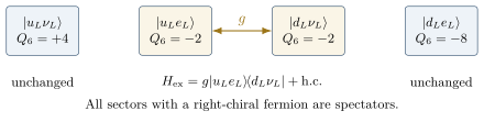
Applying UC⊗UC correctly maps ∣dLνL⟩ to ∣uLeL⟩, both of charge Q6=−2. However, it also maps ∣uLνL⟩, with Q6=4, to ∣dLeL⟩, with Q6=−8. The full commutator has
∥[UC⊗UC,Q6tot]∥2=12.(6.3)
Here ∥⋅∥2 is the spectral operator norm. A charge check on only the first input misses this failure. A single flavour flip can be used if an explicit boson or reservoir carries the compensating charge; without that resource it is not a charge-conserving closed operation.
6.3 Corrected exchange dynamics
Define Tq+=∣uL⟩⟨dL∣ and Tℓ−=∣eL⟩⟨νL∣. On the full 16-dimensional two-register space choose
Hex=gTq+⊗Tℓ−+g∗Tq−⊗Tℓ+.(6.4)
All states outside span{∣dLνL⟩,∣uLeL⟩} are spectators. The first transition raises the quark charge by six units and lowers the lepton charge by six units, so
[Hex,Q6tot]=0,[e−itHex,Q6tot]=0(6.5)
for every input and every time. Baryon and lepton number are unchanged as well. This provides a consistent finite exchange operation.
Figure 4. The corrected exchange acts only between the equal-charge states. An unrestricted pair of CNOT gates would also couple the two outer states, violating charge conservation. The displayed diagram is the left-chiral block of the full 16-state operation.
Unit transfer occurs only for a selected pulse area gt=π/2 modulo π. With detuning Δ, the transition probability becomes
P(t)=Δ2+4∣g∣24∣g∣2sin2(2tΔ2+4∣g∣2).(6.7)
The repaired gate captures a selection rule and conserved exchange. It still lacks momentum dependence, gauge fields and the spinor matrix elements needed to reproduce weak scattering or decay rates.
7 Auxiliary states, effective interactions and particle creation
7.1 A precise meaning for a virtual scratchpad
In perturbative quantum field theory, a virtual particle is represented by an internal propagator, not an independently observable asymptotic particle. Four-momentum is conserved at interaction vertices; an internal momentum need not obey the external-particle mass-shell relation [4]. Calling this a temporary violation of energy conservation is misleading.
A useful finite analogue splits a Hilbert space with projectors P and Q=I−P into retained and auxiliary sectors:
H=(HPPHQPHPQHQQ),∣ψ⟩=(ψPψQ).(7.1)
Solving the auxiliary row of Hψ=Eψ gives ψQ=(E−HQQ)−1HQPψP whenever the inverse exists. Substitution into the retained row gives the exact stationary equation
This is the Feshbach–Schur reduction [14]. The self-energy term contains the effect of auxiliary amplitudes without assigning them independent external pointers. It is generally energy dependent; replacing it by a constant Hamiltonian for all times needs an approximation or a controlled block diagonalization [15].
If the auxiliary block is separated by a gap ε and the coupling is small, the leading correction near E=0 is
Heff≃HPP−HPQHQQ−1HQP.(7.3)
A positive excitation penalty suppresses auxiliary occupation. The term “borrow stack” can denote the level counter for that penalty, but total energy is always governed by the full time-independent Hamiltonian. Auxiliary amplitudes can affect measured interference and scattering even though they are not independent detector events. Defining a detector to vanish on Q merely specifies an observable; it does not prove that all effects of Q are unobservable.
Figure 5. Effective interaction by auxiliary-sector elimination. The four-step creation protocol is a separate computational choice using preallocated resources. It is not implied by the Schur identity or by the number of vertices in a Feynman diagram.
The lower eigenvalue is negative. The original five-state electron sector has the same issue: its default lowest eigenvalue is approximately −0.073405 in model units, and the prototype reports its absolute value as a positive “derived mass”. Taking an absolute value is not a derivation of a rest mass.
A physical excitation energy must be measured relative to a consistently defined interacting vacuum. A relativistic mass additionally requires a dispersion relation, such as E(p)2−p2=m2, or an appropriately defined propagator pole. For confined quarks, mass definitions also depend on renormalization conventions. In the Standard Model charged fermion masses are associated with Yukawa couplings and electroweak symmetry breaking [10, 13]. The finite Schur model does not replace that mechanism. The corrected reference code returns energy shifts with their signs and makes no mass identification.
7.3 Real emission and reversible allocation
An isolated on-shell massive particle cannot radiate a nonzero real photon while remaining the same on-shell particle in vacuum. If p=p′+k, p2=p′2=m2 and k2=0, then p′⋅k=0. In the rest frame of p′, this would require mk0=0, contradicting a positive-energy photon. This argument is general; a census on the finite momentum grid {−1,0,1}3 is only an illustration.
Radiation can occur when another system absorbs recoil, when an initial state has excitation energy, or through other allowed scattering and decay channels. A third body is therefore one mechanism, not a universal requirement for real-particle creation. The following protocol is suitable for a recoil-assisted finite example:
Include the recoil and energy source in the total state.
Reserve a blank internal register in a preallocated pool.
Encode the outgoing pointer and entangle it with the participating systems.
Uncompute work registers when the constraints permit a completed transition.
Allocation and deallocation must retain reversibility; uncomputation is possible only if the ancillary information has been coherently accounted for. A projection onto a successful “commit” subspace is a measurement with a success probability, not a deterministic unitary reset. One may define a committed sector by kaux=0 and an increased occupation counter, but these are protocol conventions rather than universal criteria for real particles. The memory cost and gate depth depend on the chosen encoding and controller, not solely on the number of conceptual stages.
8 The generation qutrit and the charged-lepton mass ansatz
8.1 An algebraic identity with a positivity condition
For three positive masses define
K=(me+mμ+mτ)2me+mμ+mτ.(8.1)
Koide’s phenomenological relation is K=2/3[16]. Its geometric interpretation and phase parametrizations predate HQSM [17, 18]; neither the relation nor the phase near 2/9 is claimed as a new discovery here.
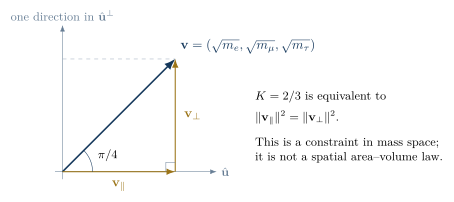
Let v=(me,mμ,mτ)T and u^=(1,1,1)T/3. Decompose v=v∥+v⊥ relative to this axis. Then
Thus K=2/3 is equivalent to equal squared norms in the one-dimensional symmetric subspace and its two-dimensional orthogonal complement. It is also equivalent to an angle π/4 between v and u^. Equal norms are an extra constraint; they do not follow from counting one radial and two tangential spatial directions. In fact, equal variance per orthonormal component would give a 1:2 norm ratio, not equal norms. Areas and volumes also have different physical dimensions, so literal fractions of area and volume cannot be equated without a separate dimensionally consistent model.
Figure 6. Koide geometry in the plane spanned by v and the symmetric axis. Equality of the two projected norms is equivalent to the mass relation. The two-dimensional orthogonal subspace of the full three-component mass space is represented by one direction in this drawing.
A qutrit clock supplies the parametrization
rg=a[1+2cos(2πg/3+δ)],mg=rg2,g=0,1,2,(8.3)
where a>0 has units of the square root of mass. The sums of the three cosines and their squares are zero and 3/2, respectively, so
g∑rg=3a,g∑rg2=6a2.(8.4)
However, mg=∣rg∣. Equations (8.4) therefore imply the physical Koide identity only when the three amplitudes are nonnegative. One positive branch is ∣δ∣≤π/12, with the other branches related by permutations. For 0<δ<π/12, the ordering (e,μ,τ) corresponds to g=(1,2,0).
At δ=π/3, one amplitude is negative. The signed ratio ∑rg2/(∑rg)2 remains 2/3, but the physical ratio is
K=(1+22)26≃0.4094.(8.5)
The original all-phase test used signed amplitudes in the denominator and therefore tested a different identity. The corrected implementation uses the principal nonnegative square roots and includes this counterexample.
8.2 Testing the fixed phase and making calibration explicit
The numerical proposal δ=2/9 radians is not fixed by the ratio of two spatial dimensions to nine two-qutrit states. No Hamiltonian, symmetry or variational principle has been supplied that selects this angle. Moreover, taking it as an exact prediction gives
memμδ=2/9=206.7703159727,(8.6)
whereas the 2022 CODATA ratio is 206.7682827±0.0000046[19]. The relative residual is 9.83×10⁻⁶, about 442 quoted standard uncertainties. This is a discrepancy, not precision agreement. The count assumes the fixed-phase formula has no theory uncertainty; introducing unspecified corrections removes its status as an exact prediction.
A consistent phenomenological repair treats both a and δ as calibrated parameters. We fix me=0.51099895000 MeV from the specified PDG electron listing [20] and solve for the phase using the independent muon–electron ratio. On the positive branch this gives
This is a two-input fit, including the overall scale. The remaining conditional prediction is mτ=1776.9690248 MeV. It is precisely the large-root Koide estimate from the two lighter masses, as can be seen without introducing a clock:
mτ=2(me+mμ)+3(me+mμ+4memμ).(8.8)
Table 3. Fixed-phase and calibrated versions of the ansatz. Data are frozen to the named sources for reproducibility; they are not inferred from the schematic figure. “Input” means the quantity calibrates a parameter.
Quantity
δ=2/9
Calibrated phase
Reference value
me (MeV)
Input
Input
0.51099895000(15)
mμ/me
206.77031597
Input
206.7682827(46)
mτ (MeV)
1776.9849684
1776.9690248
1776.93(9)
Muon-ratio residual / σ
442.02
Fitted
—
Tau residual / σ
0.61
0.43
—
The tau datum is the PDG 2025 average [21]. Propagating the ratio uncertainty with me fixed gives about 0.0000361 MeV uncertainty on the conditional tau prediction, much smaller than the 0.09 MeV experimental uncertainty. This propagation does not assign a theory uncertainty to the Koide ansatz. The experimental central values give K≃0.66666446. Agreement of the calibrated ansatz with the tau mass is an interesting empirical property; it is not a derivation of lepton masses, of exactly three generations, or of the HQSM dynamics. The distinction between pole masses and scale-dependent running masses must also be specified before testing radiative stability.
8.3 What a neutrino qutrit must reproduce
A three-level Hamiltonian conjugated by the discrete Fourier matrix can produce flavour transitions. Unitarity guarantees that its probabilities sum to one, but does not make it a neutrino model. In vacuum the ultrarelativistic oscillation amplitude has the form
Aα→β(L,E)=j=1∑3UβjUαj∗exp(−i2Emj2L),(8.9)
with mixing matrix U, measured mass-squared differences and appropriate matter corrections [22]. A Fourier matrix and three arbitrarily chosen clock frequencies are illustrative choices, not a determination of these parameters. Electrical neutrality alone does not imply oscillations or prevent decay. A proposed neutrino sector must recover the observed L/E dependence, mixing angles and mass-squared splittings.
9 Weighted chord maps and the proposed gravitational interpretation
Let ϕv and b be dimensionless potential and frame-bias parameters, and define
All exponents must be dimensionless. If ϕ or a physical acceleration is inserted, appropriate energy, length and time scales must be supplied; an acceleration cannot simply be added to a dimensionless exponent. The weights are taken as prescribed classical parameters in this section. Making them depend on an unknown quantum state’s expectation values would require a separate mean-field or fully quantum dynamical specification.
Proposition 9.1 (Convexity and the antipodal identity). For unit endpoint vectors and finite positive weights, ∥xW∥≤1, with strict inequality for distinct endpoints. For w=vˉ antipodal to v,
xW(v,vˉ)=tanhξr(v),ξ=21(sv−svˉ).(9.2)
Proof. Put λ=Wv/(Wv+Ww)∈(0,1). Then
∥λr(v)+(1−λ)r(w)∥2=1−λ(1−λ)∥r(v)−r(w)∥2.(9.3)
For antipodal endpoints the coefficient of r(v) is (esv−esvˉ)/(esv+esvˉ)=tanhξ. ◻
Coincident endpoints remain on the boundary; they are an exception to any claim of a strictly interior position for every chord. A bounded spatial coordinate is also not a causal horizon. Event horizons, Rindler horizons and de Sitter horizons require a spacetime metric and a causal structure [23]. Equation (9.2) alone supplies neither.
The prototype chooses a discrete potential
ϕ=−L+(E−Eˉ1),(9.4)
where L+ is the Moore–Penrose inverse of the cube Laplacian. Subtracting the mean makes the source orthogonal to the constant zero mode. This is a finite graph Poisson prescription. Its sign, normalization and connection to physical energy are choices to be justified by a subsequent dynamical theory.
Only differences of the sv matter. Therefore two choices satisfying
−βϕv=b⋅r(v)+c(9.5)
give identical weighted positions. This explains why a matched potential and frame bias agree to machine precision in the prototype. It is an identity of the map, not a derivation of the equivalence principle. Likewise, changing the coordinates assigned to a prescribed path can bend its plotted trajectory without demonstrating gravitational light bending. A physical prediction requires a propagation law, a metric, an operational definition of angles and clocks, and a comparison with observations such as redshift, time delay and deflection. No Einstein equation follows from the present convexity argument.
10 Reproducibility and validation
The archived software release [24] contains the four original verification scripts, their captured outputs and SHA-256 source hashes, plus a separate corrected reference implementation. The original scripts were run without modification on 5 November 2026 and reported 43 passing checks in total. These counts reproduce the programs’ own assertions; they do not endorse all interpretations in their comments or output labels.
Table 4. Original suite results and their evidential scope. Short labels map to the complete filenames in the software archive’s manifest.
Suite
Result
Scope of the passing checks
Distributed ledger
9/9
Specified code, logical operators and selected encoded Bell experiments
Stack machine
10/10
Finite register algebra, chosen self-energy matrices and weighted maps
Virtual/real compilation
12/12
Selected transitions, algebraic sums and originally implemented phase tests
Boundary atom benchmark
12/12
Finite interacting matrices, flux enumeration and encoding identities
The revised verification/hqsm_reference.py implements the mathematical definitions used here. The independent driver verification/verify_paper.py reports 23 passing checks. It enumerates the qubit and qutrit codes, tests every nonidentity one-site Weyl operator, checks all 64 chord radii and the mean-position correction, verifies radial intertwining, and tests the repaired exchange on the full state space. It also retains the nonconserving CNOT pair and the signed-root phase example as regression counterexamples. The mass inputs, fitted parameters and conditional residuals are saved in machine-readable JSON.
The recorded environment is Python 3.13.7, NumPy 2.4.4 and SciPy 1.17.1. Finite-field code calculations are exact integer arithmetic; matrix and trigonometric checks use double precision with tolerance 10−12 where appropriate. The accompanying README gives commands and pinned versions. Numbers in the mass table use explicit frozen data inputs, not values silently downloaded at execution time.
A passing original mass test, for example, only means its residual met its programmed tolerance. It did not compare that residual to the experimental uncertainty. The new tests make this distinction explicit. Similarly, testing one charge-balanced transition does not replace the full commutator check, and radial refinement of one chosen finite potential does not establish convergence to continuum hydrogen.
11 Research programme and conclusion
The finite HQSM construction has a coherent computational core: independent internal and spatial encodings, explicit erasure-correcting ledgers, reversible register operations, an exactly compressed hopping law and charge-conserving exchange dynamics. Effective interactions can be derived within a stated auxiliary-sector model. These are useful, reproducible objects for studying quantum information and simulation.
Connecting this architecture to particle physics requires several further results. A growing family of boundary graphs must have a specified continuum limit, resource scaling and physical locality. An interacting Hamiltonian must implement gauge constraints, spin and statistics, and recover relativistic dispersion and scattering. Finite gauge encodings can be studied in established quantum-link frameworks [25], but replacing SU(3) by triality alone is insufficient. A mass model must define its vacuum, symmetry-breaking structure, renormalization scheme and parameters before confronting independent data. A gravitational extension must supply dynamics and a metric rather than only a coordinate map.
The immediate falsifiable targets are correspondingly concrete: test operator conservation on every sector; measure encoding and truncation errors; demonstrate convergence of spectra and propagation on refined graphs; predict an observable not used for calibration; and verify that the prediction survives changes of regulator. The exact fixed phase 2/9 already fails the precision muon-ratio test. The calibrated Koide ansatz remains an empirical relation whose origin is unexplained.
HQSM is therefore presented as a finite boundary-encoded quantum model, not as an established replacement for the Standard Model or general relativity. Its most productive feature is the ability to state proposed mechanisms as operators and test them. The corrections developed here preserve that architectural idea while making its mathematical content, physical assumptions and outstanding obligations explicit.
Code and data availability. The supporting Python code, verification outputs and unmodified prototype snapshots are archived on Zenodo under the concept DOI 10.5281/zenodo.23991264 (all versions). The calculations reported here use release 1.0.0, 10.5281/zenodo.23991265, distributed under the MIT License [24]. The manuscript, LaTeX source, editable TikZ diagrams and supplied overview image are archived at 10.5281/zenodo.23991267 under CC BY 4.0. Particle-data inputs are identified in section 8 and the bibliography.
A Details of the stabilizer codes
For either matrix Gd, its rank is three and its row space Cd obeys Cd⊆Cd⊥. Thus dimCd⊥=8−3=5 and the quotient Cd⊥/Cd has dimension two over Fd, giving d2 cosets. The states in (4.4) are invariant under X(c) for every c∈Cd, because adding c permutes the summation. They are invariant under Z(c) because c⋅(c′+ℓ)=0 for c′∈Cd and ℓ∈Cd⊥. Distinct cosets have disjoint computational-basis supports, establishing orthonormality.
Every column of Gd is nonzero. Consider a nonidentity one-site Weyl operator Eu=XuaZub. If a=0, some Z(Gd,i) commutes with Eu only up to a phase ωk=1. If a=0 then b=0 and an X-type generator has the same property. For that stabilizer S,
Vd†EuVd=Vd†S†EuSVd=ωkVd†EuVd,(A.1)
forcing the compression to vanish. The argument works for every logical matrix element, not only for a sample of encoded pure states.
In the binary code, the vector (1,1,0,0,0,0,0,0) belongs to C2⊥∖C2. Every nonzero word of C2 has weight four or eight, so this weight-two operator is logical. In the ternary code, (0,0,0,0,0,0,1,1) is orthogonal to all three rows but is not in C3. Indeed, a nonzero combination of the first two rows alone has weight at least three; a combination with a nonzero third-row coefficient has weight six. These witnesses, together with the absence of weight-one logical operators, establish distance exactly two.
For a known-site erasure, the error products Ei†Ej span all operators on that site. The Knill–Laflamme condition is
V†Ei†EjV=αijIL.(A.2)
Equation (4.5) proves this condition for the specified codes. In a general erasure-correcting code, it guarantees a logical-state-independent local density matrix, which may be nonuniform. For instance, appending a fixed ancillary qubit ∣0⟩ to a code leaves that ancilla’s reduced state pure while providing no information about the logical state. Maximal mixing therefore requires the additional property proved above.
B Hamming-shell hopping and positional moments
Fix the anchor v and write the normalized uniform shell state as
∣m;v⟩=(m3)−1/2w:d(v,w)=m∑∣w⟩.(B.1)
Each vertex of the m shell has 3−m neighbours in shell m+1 and m neighbours in shell m−1. Counting edges gives
There are no edges within a fixed shell. Substituting n=3−m and L=3I−A gives (3.6). Uniform amplitudes within each shell remain uniform under hopping, so the encoded subspace is invariant, not merely a space onto which one may project after evolution.
The variance of the full midpoint vector in an encoded basis state is
⟨∥X−⟨X⟩∥2⟩=⟨R2⟩−∥⟨X⟩∥2=3n−9n2=9n(3−n).(B.3)
It is nonzero on the two intermediate shells. This explains how every constituent chord can have the same radius while their mean position has a smaller norm. Compression also need not preserve products of observables: V†X2V generally differs from (V†XV)2 when X maps states outside the code subspace. Care is therefore needed when constructing a spatial metric from compressed operators.
The cube spectrum follows directly from the binary characters fk(v)=(−1)k⋅v with k∈{0,1}3. Flipping coordinate i multiplies fk by (−1)ki, so Lfk=2∣k∣fk, where ∣k∣ is the Hamming weight of k. This gives eigenvalues 2∣k∣ and multiplicities (∣k∣3). It supplies an exact finite angular spectrum while making its difference from continuum spherical harmonics explicit.
C Logical no-signalling and the Bell bound
Let EA(ρ)=∑rKrρKr† with ∑rKr†Kr=IA. For any observable B of the second logical subsystem,
All expectation values of B are unchanged, proving (4.9). Selecting a single r breaks the completeness sum and describes conditioning, not a signalling channel without the outcome record.
For dichotomic observables Ai2=Bj2=I on separate factors, define S=A0⊗(B0+B1)+A1⊗(B0−B1). Expanding gives
S2=4I−[A0,A1]⊗[B0,B1].(C.2)
Each commutator has operator norm at most two, hence ∥S∥≤22. The singlet and observables in section 4 attain this bound. An isometric encoding preserves their logical expectation values. These statements are consequences of the assumed quantum tensor-product structure, not of the pointer geometry.
D Controlled elimination and error estimates
Suppose HQQ≥εI with ε>0. For real E<ε, the inverse in (7.2) is negative definite. Thus the self-energy is negative semidefinite on the retained subspace. This sign check rules out interpreting every downward shift from a zero diagonal entry as a positive rest energy.
In the two-state example, rationalizing the square root gives
The last inequality is a concrete remainder bound for the leading effective interaction. It is stronger than describing the correction as “small” without a scale.
For a more general dynamical approximation, let H and HB be self-adjoint and V an isometry. If ∥HV−VHB∥≤ϵ, differentiating the product of propagators and integrating gives
∥e−itHV−Ve−itHB∥≤∣t∣ϵ.(D.2)
This identifies the residual and time interval that a numerical encoding test must control. It does not imply that an energy-dependent Schur complement is an exact time-local Hamiltonian at every energy.
E Mass calibration and interpretation of residuals
For the ordering (e,μ,τ)=(g=1,2,0), define
F(δ)=[1+2cos(2π/3+δ)1+2cos(4π/3+δ)]2.(E.1)
On 0<δ<π/12, the numerator increases and the positive denominator decreases, so F is strictly increasing. It starts at one and diverges at the upper endpoint. There is therefore one solution for every measured ratio greater than one. The reference implementation brackets this root; the electron mass then fixes a. There is no unreported phase-selection freedom within this chosen ordering and branch.
Near the fitted phase, dlogF/dδ is about 56 per radian. The difference between 2/9 and the fitted phase is only 1.75×10⁻⁷ radians, yet it produces a roughly 9.83 parts-per-million mass-ratio residual. A small phase difference is not small compared with the measurement precision. The 442-standard-uncertainty comparison in section 8 tests the fixed formula; it is not a goodness-of-fit claim for a model with unknown correction terms. Once δ is calibrated, the muon datum cannot also count as an independent successful prediction.
F Computer-science and physics terminology
Table 5. Terminology used in this paper. Each analogy has a specific mathematical meaning.
Architectural term
Mathematical object
Boundary of the analogy
Species definition
Fixed classical table of representations and couplings
Does not imply a shared mutable quantum state
Ledger
Encoded logical subsystem VdLd
Finite capacity; local marginal protection applies only to this subsystem
Pointer
Boundary-address state ∣v,w⟩
Distinct addresses can have the same midpoint
Stack
Integer or modular counter with reversible shifts
Does not store a last-in–first-out history by itself
Message bus
A charge-conserving coupling between sectors
Does not reproduce a gauge field merely by being spin one
Scratchpad
Auxiliary subspace QH
Its effects survive elimination; energy is conserved in the full system
Commit
A designated output sector with cleared work registers
A postselected success is not a deterministic reset
Generation clock
Three-level spectral parametrization
Three generations and parameter values remain assumptions
Holographic lens
Positive-weight chord barycenter
A coordinate map is not a spacetime metric or a gravitational dynamics
References
R. P. Feynman. “Simulating physics with computers”. In: International Journal of Theoretical Physics 21 (1982), pp. 467–488. doi:10.1007/BF02650179.
J. M. Maldacena. “The Large N Limit of Superconformal Field Theories and Supergravity”. In: Advances in Theoretical and Mathematical Physics 2 (1998), pp. 231–252. doi:10.4310/ATMP.1998.v2.n2.a1. arXiv:hep-th/9711200.
A. Almheiri, X. Dong, and D. Harlow. “Bulk locality and quantum error correction in AdS/CFT”. In: Journal of High Energy Physics 2015.4, 163 (2015). doi:10.1007/JHEP04(2015)163. arXiv:1411.7041.
D. Tong. Lectures on Quantum Field Theory. Author’s lecture notes; especially sections 2–6. University of Cambridge. https://www.damtp.cam.ac.uk/user/tong/qft.htm (visited on 5 November 2026).
W. K. Wootters and W. H. Zurek. “A single quantum cannot be cloned”. In: Nature 299 (1982), pp. 802–803. doi:10.1038/299802a0.
D. Gottesman. “Stabilizer Codes and Quantum Error Correction”. PhD thesis. California Institute of Technology, 1997. arXiv:quant-ph/9705052.
J. F. Clauser, M. A. Horne, A. Shimony, and R. A. Holt. “Proposed Experiment to Test Local Hidden-Variable Theories”. In: Physical Review Letters 23 (1969), pp. 880–884. doi:10.1103/PhysRevLett.23.880.
C. S. Wu, E. Ambler, R. W. Hayward, D. D. Hoppes, and R. P. Hudson. “Experimental Test of Parity Conservation in Beta Decay”. In: Physical Review 105 (1957), pp. 1413–1415. doi:10.1103/PhysRev.105.1413.
G. Dusson, I. M. Sigal, and B. Stamm. The Feshbach–Schur map and perturbation theory. 2021. arXiv:2105.02058.
S. Bravyi, D. P. DiVincenzo, and D. Loss. “Schrieffer–Wolff transformation for quantum many-body systems”. In: Annals of Physics 326 (2011), pp. 2793–2826. doi:10.1016/j.aop.2011.06.004. arXiv:1105.0675.
Y. Koide. “New view of quark and lepton mass hierarchy”. In: Physical Review D 28 (1983). Erratum: Phys. Rev. D 29, 1544 (1984), pp. 252–254. doi:10.1103/PhysRevD.28.252.
P. Żenczykowski. “A Note on Koide’s Doubly Special Parametrization of Quark Masses”. In: Open Physics 16 (2018), pp. 427–429. doi:10.1515/phys-2018-0058.
National Institute of Standards and Technology. Muon–electron mass ratio: 2022 CODATA recommended value. 206.7682827(46). https://physics.nist.gov/cgi-bin/cuu/Value?mmusme (visited on 5 November 2026).
The version of record is archived on Zenodo at the DOI above; this page and PDF are the publisher copies at neusym.ai.
See the full list of papers for the rest of the programme.