Fermions and Colour: Transport and its limits in qutrit–qubit networks
David Elliman · Neuro-Symbolic Ltd · 5 November 2026
Summary and scope
The quantum state of two fermions, such as quarks, changes sign when they are exchanged, and quarks also carry a three-valued internal label called colour. Can networks of small quantum registers reproduce both features? We build each site from four qutrits (three-level quantum systems). Its lowest-energy states record whether the site is occupied and carry a three-component SU(3) colour. Moving the occupation, carrying the colour and obtaining the fermion sign turn out to be separate requirements. Interactions that swap pairs of qutrits move a particle only indirectly, through brief virtual visits to higher-energy states; the same processes also create particle pairs and unwanted colour-dependent returns. A cancellation that removes these on one isolated link fails where links meet, because different links share virtual states. The fermion sign can instead come from preparing the empty sites in an antisymmetric colour state, using a known correspondence between internal symmetry and particle statistics. This needs shared entanglement, allows at most three empty sites, and is not singled out by the hopping Hamiltonian. Adding colour-neutral auxiliary registers keeps the virtual processes on different links apart. Six existing Hamiltonian parameters are then fixed from single-link equations, without fitting masses, mixing angles or propagation scores. At an operating point chosen in advance, a simplified (effective) model of a four-site junction gives minimum fidelity 0.99499 with ideal fermion hopping and maximum leakage out of the encoded states of 0.207%, over sixteen hop times on 102 tested states. A separate implementation reproduces these results. A point with a smaller energy penalty on pair creation fails the same sixteen-hop test. Virtual creation and removal of particle pairs explain, to leading order, the remaining coherent error. A residual calculation bounds the difference between this effective model and the full four-site Hamiltonian. For the same sampled test it gives microscopic fidelity at least 0.99375 and leakage at most 0.326%. The bound is evaluated numerically, without interval certification. This is a finite-model result: the interactions still require supplied three-register controls, precisely calibrated parameters and a prepared background state. Scalable preparation, robustness and a complete microscopic theory of fermions remain open.
Keywords
How to cite
Elliman, D. (2026). Fermions and Colour: Transport and its limits in qutrit–qubit networks. Neuro-Symbolic Ltd technical report. https://doi.org/10.5281/zenodo.23974020
@techreport{elliman2026fermionscolour,
  author      = {Elliman, David},
  title       = {Fermions and Colour: Transport and its limits in qutrit–qubit networks},
  institution = {Neuro-Symbolic Ltd},
  year        = {2026},
  doi         = {10.5281/zenodo.23974020},
  url         = {https://neusym.ai/papers/fermions_colour/}
}
Full text
The complete paper, rendered as HTML with the mathematics set at build time. The PDF above is the typeset version of record; equation, theorem and reference numbers match it.
Finite-model research draft with independent computational checks. The microscopic bounds are numerical and restricted to the stated experiment; human peer review remains pending.
1 What must a coloured particle do?
This paper asks a deliberately limited question. Suppose we build a small network out of quantum registers (finite-dimensional quantum systems, the quantum analogue of memory cells). Can a pattern in that network behave like a moving particle that carries an internal “colour” label and obeys the exchange rule of fermions (particles such as electrons and quarks, whose joint quantum state changes sign when two of them are swapped)? These questions can be studied in finite quantum systems without assuming that the systems already describe elementary particles.
A useful microscopic model of a moving particle must do more than transfer an excitation between two registers. It must specify three things: what counts as a particle, which internal state moves with it, and how two particles behave when their paths exchange.
Here a qutrit is a three-dimensional quantum register, that is, a quantum system with three basis states. When we call it a fundamental colour register, we mean that a colour rotation acts on it as the three-dimensional representation . (The group is the set of unitary matrices with unit determinant; it is the symmetry group of colour in the strong interaction. A representation is a rule assigning a matrix to each group element, and is the basic three-dimensional one, also called the fundamental or triplet representation.) Colour is an internal quantum label. It is not a spatial direction, and global covariance alone is not a local gauge theory of quantum chromodynamics: we only require that the model treats all colour rotations, applied everywhere at once, as symmetries. A qubit is a two-dimensional register; it can supply the binary grading (the even/odd bookkeeping) used in a fermionic encoding. Neither register’s dimension, by itself, determines the statistics of a collective excitation.
The model studied below distinguishes three operations, each of which can succeed or fail independently:
Occupation transport: a two-valued label changes from to on neighbouring blocks. In words, “particle here, none there” becomes “none here, particle there”.
Colour transport: the colour associated with the occupied block follows that change.
Fermionic exchange: two nonzero sequences of legal hops differ by a minus sign after their final internal states are identified consistently.
The third condition concerns an interference experiment: two different routes lead to the same final arrangement, and the fermion sign is the relative sign between them. Multiplying every hopping amplitude by does not impose it: two histories containing the same three links acquire the same three scalar factors, so their relative sign is unchanged.

Finite-register descriptions of gauge fields and quantum information have a substantial history. Qutrit codes provide useful finite state spaces[1]; Hamiltonian lattice gauge theory and gauge magnets specify how local constraints relate matter and links[2, 3]. Our question is narrower: what does a particular static, -invariant pair-exchange Hamiltonian actually generate in a selected low-energy subspace? Here “pair exchange” means an interaction built only from operators that swap the states of two registers, and “static” means that the Hamiltonian is fixed rather than switched on and off in time. The use of representation multiplicities (repeated copies of the same representation) for encoding is related to exchange-only quantum computation[4], but a sequence of controlled gates is not the same construction as one fixed Hamiltonian.
The statistics benchmarks likewise use established ideas. Jordan–Wigner, Bravyi–Kitaev and related encodings represent fermions by spin operators[5–9]. Levin and Wen formulate statistics directly in terms of hopping operators[10]. Gauge constraints and string operators can produce fermionic excitations in bosonic microscopic systems[11–13]. We use these results as reference constructions; the existence of a minus sign after a prescribed string dressing (an extra operator attached along the particle’s path) is not a new derivation of fermions from qutrit exchange.
The contribution of this paper is the analysis of one particular pair-exchange law: its virtual hopping coefficients, an isolated-link cancelling family, the failure of that cancellation at a junction, and a tuned auxiliary extension. The exchange sign obtained from an antisymmetric colour background is an application of known colour–orbital symmetry relations, not a new statistics mechanism. The corresponding occupancy limit is also known[14]; entangled-photon experiments have simulated the associated bosonic and fermionic interference[15, 16].
The presentation follows the physical construction. Sections 2–4 build the basic unit (a “block” of four qutrits) and work out which couplings between blocks make a particle move. Sections 5–6 explain the exchange test and show that the state of the empty blocks decides whether it can be passed. Section 7 realizes the relational code on fixed site registers, explains its preparation and scaling costs, and reports the qualified auxiliary-junction result, including numerical error bounds. Appendix D keeps the finite rotation diagnostics separate from dynamical exchange.
2 A block with occupation and colour
This section builds the basic unit of the model. The aim is a small group of qutrits whose lowest-energy states can be read as “empty” or “occupied”, while also carrying one complete colour triplet. We first find such states using symmetry, then fix a convention for which of them counts as occupied, and finally give a Hamiltonian that makes them the ground states.
2.1 Two copies of a colour triplet
Each block contains four fundamental qutrits, labelled . Its Hilbert space (the space of all its quantum states) is
Schur–Weyl duality separates the colour representation from the multiplicity with which it occurs[17]. This theorem says that the 81 states of four qutrits split into pieces, each of which is a colour representation of paired with a representation of the permutations of the four qutrits; the permutation part counts how many equivalent copies of that colour representation there are. To avoid ambiguous names for the two 15-dimensional representations, we label colour representations by their Dynkin indices (the standard pair of integers that identifies an representation):
An explicit triplet embedding makes this statement concrete. Define a normalized antisymmetric pair by
2.2 Fixing the occupation convention
The two-state label can be described in several bases, and choosing the wrong one later leads to a wrong hopping operator. This subsection fixes the convention once and for all. Let denote Pauli matrices in the copy basis . Direct permutation of the qutrits gives
Both and transform as colour triplets. Calling “empty” therefore does not make it a colour-singlet vacuum: an empty block still carries a colour. This distinction will be decisive in Section 6.
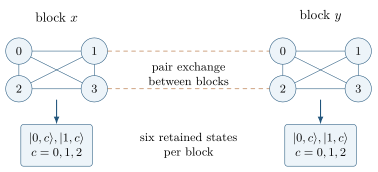
2.3 An isolated six-state ground space
An energy gap is needed before virtual-transition calculations are meaningful. We therefore want a Hamiltonian on each block, built from pair swaps, whose lowest-energy states are exactly the six code states and which separates them from all other states by a finite energy. Define the class sum and the pair operator
The fixed selector used here is
3 What pair exchange actually generates
We now couple two blocks with pair swaps between their qutrits and ask what effective motion results inside the code space. The short answer is: at first order in the coupling, colours can be exchanged but the particle cannot move; at second order, through brief visits to higher-energy states, it can move, but other unwanted processes (such as creating two particles at once) appear at the same order.
3.1 First order: colour exchange without occupation motion
Take two blocks, and , with . Let , with the encoded factors reordered as occupation–occupation–colour–colour, and let , . Here projects onto the code space of the two blocks and onto everything else. We write encoded matrices as rather than confusing them with physical-space projections.
To compute what a physical operator does inside the code, we need its compression , the part of that acts within the code space. The local colour matrix unit (which changes colour to colour on qutrit ) has compression
For example, take and
There is also a quantitative first-order limitation, which shows that no choice of pair couplings can produce the target hop at first order. The identity and all 28 pair swaps on eight physical qutrits compress to a nine-dimensional operator space. Adding the target in Eq. (9) raises the rank to ten. The matrix is orthogonal to that entire pair span under the trace inner product, whereas
3.2 Second order: virtual excursions enable motion
Higher-order processes work through virtual excursions: the coupling briefly takes the system out of the code space into a higher-energy state, and a second application brings it back, possibly in a different code state. Such two-step processes are suppressed by the energy cost of the intermediate state but can do things a single step cannot.
We measure energies in one fixed reference unit and set . The inherited numerical coupling is . This is an input, not a mass prediction. To distinguish perturbative order from an energy scale, write , with dimensionless expansion parameter . For the first-order-silent couplings below (those with zero first-order effect in the code),
For a real port vector , define . A port vector is simply a set of four weights saying how strongly each qutrit of a block takes part in the coupling. The vectors
| Occupation block of | ||
|---|---|---|
| , | ||
| , | ||
| Single-occupation flips |
Table 1 gives the complete block structure for . Its rows are, in order: hopping (), pair creation or annihilation (), energy shifts of configurations with equal occupations, energy shifts with unequal occupations, and processes that change only one occupation. The coefficients were calculated by an exact rational solve in the 560-dimensional physical colour-weight sector (the states containing three qutrits of each of two colours and two of the third). This sector contains both colour arrangements needed to determine and ; covariance then determines the nine-dimensional colour operator. It is a symmetry reduction of the two-block problem, not a claim that a dense 6561-state time evolution was run.
For or alone, both the hop and pair block equal , but there are also eight nonzero single-flip blocks. Their coefficients have magnitudes corresponding to , with signs depending on the block. Those terms cannot be discarded when checking occupation constraints.
It is essential to distinguish two parity statements. Matter parity is whether the total number of particles is even or odd; fermion models normally require it to be conserved. The question is whether that conservation holds only at the order computed, or exactly. Define the physical involution , whose code action is . Then
3.3 Finite gaps and the limits of the effective law
The second-order formula is only the first term of a series. The exact energy-dependent return operator, which includes every order, is
The transport calculations retain the declared colour-weight sectors. The clock Hamiltonian and its three coherent spectator blocks from Ref. [20] are not part of the junction Hamiltonian studied here. The spectator particles tested below are a different extension.
4 Two hopping channels
The previous section showed that second-order hopping exists but, for the simple couplings tried, always drags along an unwanted identity term . This section explains why, using symmetry, and then shows how a more elaborate coupling can cancel on a single link, and why that cancellation breaks down once several links meet at a junction.
4.1 A symmetry explanation of the fixed ratios
Four real vectors form a basis for the site weights on a block:
The selector commutes with both and . Each occupation state has definite eigenvalues under these swaps: for and for . Changing occupation therefore reverses both signs. Under conjugation, the port vectors carry the characters shown in Table 2.
| Port | ||||
|---|---|---|---|---|
| Character under |
Since the excited-state resolvent preserves these characters, a second-order hop can contain only followed by , or the reverse, on each block. This is a selection rule: symmetry alone forbids most processes. Of the 256 ordered pairs of port products, 192 cannot connect any two code states and vanish exactly. Of the remaining 64, 55 are nonzero in at least one occupation block. The selection rule fixes which processes can occur; their nonzero sizes still depend on the virtual energies.
For every coefficient matrix , the hopping block is
If only the first product in Eq. (26) is present, . If only the second is present, . Neither channel alone permits with . In other words, each channel on its own has a locked ratio of wanted to unwanted hopping, and neither ratio is the pure colour-carrying hop. These are exact restrictions on the fixed selector and the stated perturbative order. An antisymmetric inter-block pattern need not have zero hop: gives and obeys the second ratio.
4.2 Cancellation on one isolated link
Mixing the two channels can make vanish, but at a price. With alone, combining the two channels always generates single-occupation flips: with needs all four of to be nonzero, while zero flips would require . That does not extend to the full family. The ports and contribute to the single-flip blocks and can cancel them, even though they do not alter Eq. (26).
The following explicit real coefficient matrix cancels the identity part of the second-order hop. Order its rows and columns as , and define
This isolated-link cancellation does not supply the required protected fermion model. Its coefficients are selected to satisfy algebraic cancellation conditions, its microscopic interaction contains both parities, and its pair-creation and diagonal returns remain. An overall small in is needed for a controlled perturbative interpretation. No higher-order identity cancellation or all-order matter-parity conservation follows from Eq. (29).
Appendix B gives the complete real first-order-silent cancellation family, up to scale, discrete signs and two continuous ratios in the entries. Hop and pair blocks depend on the same two products through an invertible coefficient matrix, and vanish only together: one cannot keep the hop while removing pair creation. At , the pair block is approximately , compared with the hop . The printed pattern also has a diagonal colour coefficient about times the hop. Thus an isolated pure-swap hop block is not an isolated transport process.
The diagonal colour term also commutes with the hop. Such a term keeps rotating the colour state while the particle hops, which degrades colour transport. For a normalized input colour state , its fidelity with ideal colour exchange at the hop time is
The restriction that does survive is useful: with this selector, a coupling of definite matter-parity character has one of the locked second-order ratios. A general mixture can evade the ratio obstruction through cancellation. Exact symmetry protection and cancellation at one perturbative order are distinct design requirements.
4.3 Why the isolated-link cancellation fails at a junction
A network needs junctions, where one block is linked to several others. There, a virtual excursion can start on one link and return through a different link sharing the same block. For links and , the additional second-order operator is
For the entire real cancellation family in Appendix B, an unavoidable centre-only flip has magnitude relative to the hop
5 Testing the fermion sign at a junction
This section sets up the experiment that decides whether particles behave as fermions. On a small star-shaped network, two particles can reach the same final arrangement by two different sequences of hops. For fermions, the two routes must differ by exactly a minus sign. We describe the test, explain what an added layer of qubits can and cannot supply, and review one standard way of producing the sign.
5.1 The two paths must be physically legal
We use a central site with leaves (a four-site “star”). Let move a particle from to , and initially occupy leaves and . The two histories are
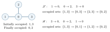
For a single internal species, the Levin–Wen criterion is on the relevant nonzero two-particle sector[10]. Directed hops are generally singular operators: a hop annihilates a state (gives zero) if the source is empty or the destination is occupied. They should not be replaced indiscriminately by globally invertible toggles, that is, by operators that simply flip occupations regardless of the current state.
5.2 What the qubit layer supplies
Qubit strings can realize the required anticommutation algebra, the defining algebraic rule of fermion operators. On the eight-vertex face-incidence graph of an octahedron, the checked reference encodings use either eight face qubits or twelve edge qubits. The local face construction has hop support at most four qubits; the edge construction has support at most five. (The support is the number of qubits a single hop operator acts on.) These are finite-graph examples of established fermion-to-spin encoding methods, particularly the superfast encoding[6, 9].
Adding qutrit-link shifts preserves the qubit exchange word and moves a three-valued detector charge. To describe a particle with a fixed charge, one must also restrict the toggle to an occupied-to-empty hop and impose the appropriate matter–link matching constraint. A bare endpoint toggle can create a pair, and is not automatically a number-preserving, gauge-invariant charged-particle hop. Nor does detector charge establish transport of an triplet: a three-valued label is not the same as a full colour state.
There is a simple reason not to overinterpret the failure of a pure-qutrit unitary ansatz. For invertible operators on one common -dimensional space,
5.3 Planar charge–flux dressing
One supplied route to the statistics sign uses planar charge–flux attachment. The idea, familiar from the toric code, is to bind a “charge” and a “flux” together: neither alone is a fermion, but the composite is. Put a qubit on each link and define commuting star and plaquette operators
For the declared shortest, non-enclosing ribbons, the monochrome sector (all four sites with the same colour) gives . With , its nonzero scalar hop is
The diagonal terms in Table 1 need no ribbon. Both hopping and pair creation flip two endpoints and can be dressed to commute with Eq. (36). A term flipping only one endpoint is incompatible with this particular two-endpoint ribbon prescription. Gauge invariance of the pair term does not establish its full mixed pair–hop statistics algebra; only the two-particle hopping comparison has been tested.
6 The state of the empty blocks
So far we have ignored a subtle point from Section 2.2: an empty block still carries a colour. This section shows that this leftover “background” colour can record which path the particles took, and so spoil the interference that defines the fermion sign. We then ask what background state avoids the problem, and find that the answer is tightly constrained by representation theory.
6.1 The exact four-register comparison
For an arbitrary colour state on the four blocks, write the colour part of one hop as . Temporarily separate the ribbon sign from the matter matrices. With the histories of Eq. (33), their matter factors are
Proposition 6.1. For the same coefficients on the three links, and , Eq. (38) satisfies a scalar-times-register-permutation identity only in the following two cases:
In words: the two histories can only be compared cleanly if the hop either never moves colour () or always moves it (), and in the second case the comparison necessarily swaps the colours of the empty sites as well as those of the particles. The proof is a finite exact polynomial classification, described in Appendix C. It covers all 24 register permutations and takes account of the one-dimensional kernel of the group algebra on four triplets. It does not classify more general state-dependent intertwining operators. Independent coefficients on the three links give further solutions, including , but that case occurs only where two links carry no colour and the third is a singular projector (), so that and no comparison of paths remains. If every link has , the only solution is still , with all .
For the derived coefficients, the best scalar fit using the double transposition has relative Frobenius residual about ; the identity comparison has residual about . These numbers are diagnostics of failure, not statistical phases. The fitted matter multiplier near is not a unit-modulus exchange phase, and the ribbon sign must still be applied separately.
6.2 What a pure swap does to the background
The branch moves occupation while leaving colour on the sites. It therefore fails the intended colour-carrying interpretation. The branch transports colour, but swaps the colour of the empty block in the opposite direction: when a particle’s colour moves forward, the empty block’s colour moves back to take its place.
Under a pure swap, the two histories in Eq. (38) induce inverse four-cycles. Acting on an initial register ordering , they give
For example, take identical red particles and distinct green and blue backgrounds:
One possible restriction is to demand that every interchange of empty registers act as a scalar on the background, so that it cannot record anything. If all empty pairs can be interchanged, the transpositions generate their full permutation group. Its one-dimensional representations are the trivial and sign representations, so the background must be totally symmetric or totally antisymmetric. For empty triplets,
6.3 A short representation-theory obstruction
The antisymmetric option is the familiar relation between internal symmetry and orbital statistics: for bosons, a state that is antisymmetric in colour must also be antisymmetric in position, so its motion carries a fermion-like sign. Herviou gives the lattice correspondence using colour and orbital representations: an antisymmetric colour sector of bosons supports the orbital sector associated with colour-symmetric fermions, with the bound that the number of antisymmetrized colours cannot exceed their dimension[14]. The limit of three empties here is that same restriction. Photonic demonstrations of statistics-dependent interference provide experimental precedents[15, 16]; they do not prepare the state or Hamiltonian of this model.
For the stronger demand that every empty-pair swap act as , the mean swap expectation must be . The lowest class-sum eigenvalues give the explicit bounds
6.4 The standard centre-charge restriction
Could a different local code make an empty block a true singlet while retaining a triplet particle? The natural single-occupancy local space would be (empty is colourless, occupied carries a triplet), rather than the present .
The following is a standard consequence of the action of the centre on tensor-product representations[17]. (The centre of consists of the three matrices that commute with every group element, namely the identity times a cube root of unity; its eigenvalue on a representation records the triality.)
Proposition 6.2 (Fixed-product triality obstruction). Under the diagonal product action of , no fixed tensor product
Proof. For , the central element acts on all of as the same scalar,
Put simply, with this symmetry action a fixed collection of triplet and antitriplet registers cannot contain both a colourless state and a triplet. This proposition fixes the symmetry action as well as the microscopic carrier. It is not a prohibition on all qutrit-based descriptions of charged matter. A relational encoding can distribute compensating charge outside the region called a site; a gauge-dressed encoding can include boundary flux; and a direct-sum local carrier can have more than one triality. Each changes a stated premise. Simply adding a colour-neutral control bit, or switching off a coupling to an empty fundamental qutrit, does not change its centre eigenvalue.
7 A local dressed junction
This section turns the lessons of Sections 4 and 6 into a working construction, and then measures how well it works. In outline: we place the empty sites in a shared antisymmetric (singlet) colour state, which supplies the fermion sign; we show that a simple local hop then reproduces fermionic hopping exactly; we discuss what this costs in entanglement and scalability; and we add auxiliary two-state systems that keep virtual processes on different links apart. Finally, we calibrate the adjustable parameters, simulate the resulting effective model, and bound its error relative to the full microscopic Hamiltonian.
7.1 Realizing the relational code on fixed registers
A relational description need not imply that one shared hardware register must be moved from site to site. Here “relational” means that the colours are recorded relative to which sites are occupied, rather than in permanently assigned registers. Keep the occupation and colour registers at fixed sites, and encode their relation in the state. For four sites and two particles, add one boundary colour qutrit, denoted , which never hops. If the occupied sites are and the empty sites are , define the isometry
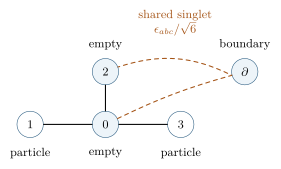
| Register | Colour representation | Function |
|---|---|---|
| Site occupation | Neutral copy label in each four-qutrit block. | |
| Site colour | Particle colour when occupied; background colour when empty. | |
| Boundary colour | Completes the shared singlet and does not hop. | |
| Two auxiliaries per link | Distinguish virtual channels in the auxiliary law. |
Each site still transforms as a triplet in either occupation state. Four physical four-qutrit blocks and one boundary qutrit contain 17 fundamentals, with centre phase , exactly the phase of the two particle colours. The construction respects Proposition 6.2; it relocates the neutral vacuum to a shared sector rather than finding a local inside one fixed block.
7.2 A local hop and its known statistics mechanism
Let move a particle from to . The operator
Reordering the empty registers after a hop changes the singlet by , because the singlet is antisymmetric. Since the number of empty and occupied sites strictly between the endpoints sums to ,
For the three-hop histories, the particle colours acquire their exchange and the two empty colours contribute . Thus, without a ribbon,
The connection to prior work can be stated as an evaluated map. Regard empties as hard-core bosons carrying colour (bosons that cannot share a site), and take identical particle colours. A particle hop is then a background-boson hop :
7.3 Preparation and scaling are physical costs
The local hop is not free: the sign comes from the prepared background, and that background has costs of its own. Equation (49) contains no string operator, but Eq. (47) requires entanglement shared by the empties and the boundary, however far apart they become. Operator locality has not supplied local state preparation. Moradi Kalarde et al. explain this distinction in their operational comparison of fermions and bosons: suitable pre-shared entanglement can enable a bosonic simulation while changing the state-preparation resources[22]. Our finite construction illustrates that cost; it does not establish their general operational theorem.
Nor does the pure hop prepare the singlet by energy minimization; that is, the desired background is not simply the lowest-energy state. With two identical-colour particles and two mobile empty registers plus one boundary qutrit, the lowest energies in the background colour sectors are:
| Graph | Hop coefficient | Singlet | Mixed | Symmetric |
|---|---|---|---|---|
| Star | ||||
| Star plus link – | ||||
| Star plus link – |
For identical particle colours the singlet-background sector is conserved but excited on the star. Allowing all particle colours gives a state at inside that sector, degenerate with other background sectors. Thus the hopping term does not uniquely prepare the desired background. In the identical-colour test, the added frustrated link only produces a tie for lowest energy. Singlet-cluster selection on frustrated bosonic lattices[14] and hole-induced singlets in particular fermionic Hubbard models[23] are leads for a preparation mechanism, not evidence that one exists here.
For empties the singlet construction adds pinned boundary qutrits. For , the required totally antisymmetric background is absent. The construction can accommodate more particles but cannot describe a dilute network with arbitrarily many empties. One may instead use a symmetric coloured background and a separate ribbon sign, but that changes the vacuum and statistics resources. Multiplying the independently established background and ribbon signs predicts a minus sign for symmetric background plus ribbon and a plus sign for antisymmetric background plus ribbon; that composition has not been simulated in this junction study.
7.4 Separate colour symmetries explain the necessary tuning
Before building the full Hamiltonian, it helps to know which unwanted terms actually threaten the singlet background. A symmetry argument answers this. Let act on the colour at site . There are separate generators for particle colour and background colour:
Write the occupation projectors on a link as
Consequently, among these number-conserving diagonal colour terms, only the unlike-occupation term needs cancellation for code invariance. This does not remove pair creation, guarantee the desired orbital energies, or protect the cancellation against higher-order returns. The numerical auxiliary study below cancelled all diagonal colour coefficients; the symmetry analysis suggests a less restrictive future design, which has not been tested dynamically.
7.5 The auxiliary Hamiltonian
Section 4.3 showed that virtual excursions returning through a different link spoil the junction. The remedy studied here is to give each link its own “flag”: two extra two-state systems (auxiliaries), one for each hopping channel, which are flipped whenever that channel’s coupling acts on that link. A process that starts on one link and returns on another would leave a flag raised, so at second order it cannot return to the low-energy space. Two neutral two-state auxiliaries on every star link distinguish its virtual channels. Let be their excitation projectors and their flips. In units of the fixed energy scale , the microscopic law to be approximated is
The remaining controls are physical pair couplings and internal swaps:
At second order the two isolated channels have coefficients
One protection does hold exactly:
7.6 Calibrating existing controls at finite coupling
The settings above cancel unwanted terms only at second order. At the finite coupling actually used, higher-order terms shift the balance. We therefore re-tune the Hamiltonian’s own adjustable parameters so that the exact single-link behaviour has the desired form. The finite-coupling construction keeps Eq. (57) and solves for its existing controls. It does not delete effective operators by hand. The two operating points , and were fixed before the new calculation. At each point six link equations determine
To define the link operator unambiguously, let embed the bare block code with all auxiliaries in their ground states on a cluster . Let contain the orthonormal code-connected eigenvectors of its physical Hamiltonian, with dimensionless eigenvalues in units . For , let be its unitary polar factor (the unitary matrix closest to ). The effective operator in bare code coordinates is
Write its occupation blocks as and set . The six conditions are
| Control | ||
|---|---|---|
The maximum equation residual is below . A separate one-link implementation reproduces the parameters to and the effective link matrices to in maximum-entry error. This is a reproducible finite-coupling calibration, not a parameter-free law or a symmetry-protected cancellation.
7.7 The effective star and its tested time window
With the controls fixed, we assemble an effective Hamiltonian for the whole four-site star from the single-link and two-link results, and compare its time evolution with ideal fermion hopping. Every cluster contains the full field on its centre and on each of its leaves. The connected two-link correction and assembled star are
Equation (66) retains pair creation and colour-dependent returns. It omits connected three-link corrections and microscopic bare-state dressing (the small admixture of excited states in the true low-energy states). Evolution uses scaled time and the finite-link colour-carrying coefficient , giving
The fixed test uses all 54 code basis states and 48 new complex superpositions, eight in each of six conserved colour-count sectors, with seed . Only the superpositions are new; the basis states had been tested before. A time grid resolves the fastest spectral phase increment to at most radians. The criterion is sampled and throughout the stated window.
| Hop times | Minimum | Maximum | Criterion | |
|---|---|---|---|---|
| 40 | 4 | Pass | ||
| 40 | 8 | Pass | ||
| 40 | 16 | Fail | ||
| 80 | 4 | Pass | ||
| 80 | 8 | Pass | ||
| 80 | 16 | Pass |
The improvement is substantial but has a finite scope. An independent prospective test (one whose pass criterion was fixed in advance) of the uncalibrated second-order settings at , gave and over eight hops on 78 starts. That failure stands; Table 6 tests different physical coefficients, fixed by Eq. (65), and a new random seed. The earlier four-hop comparisons remain valid within their shorter window. By itself, the successful calibrated point establishes sampled effective dynamics. Section 7.10 supplies the separate bound connecting it to microscopic fidelity.
7.8 Why virtual pairs still limit transport
This subsection identifies the main source of the remaining error. Even after calibration the link creates and annihilates pairs through
The leading signs have a simple explanation. Let be the gap for a centre-occupied pair to visit , and the corresponding gap for a leaf-occupied pair to visit . Neglecting smaller scalar and colour terms in these denominators gives
Since , the return adds a positive colour-swap term as well as a negative scalar shift. The return shifts the leaf-occupied configurations upwards. Returns through different links also connect different two-particle configurations and different background states; diagonal counterterms cannot remove all of them. The error amplitude therefore has a natural scale and can accumulate coherently with time. It is not a constant leakage rate.
At the mean code energy, the projected Schur-correction norm divided by is for and for . Doubling reduces the sampled sixteen-hop infidelity by and leakage by , consistent with a leading amplitude of order over this window (an amplitude error of order gives probability errors of order , hence the factor of about four). Hypothetically removing all number-changing terms raises both sixteen-hop fidelities above ; that deletion isolates the mechanism but is not an allowed physical repair.
The calibrated two-link correction has norm and in scaled energy units at the two points. Removing it changes the sixteen-hop minimum fidelity by only and , respectively. It is retained in Table 6. These small changes identify its contribution in the chosen full-field convention; they do not bound omitted three-link effects.
7.9 Bounding the dressing of the full star
The simulations above use the effective model, not the full microscopic Hamiltonian. The remaining subsections ask how far the two can differ, and derive bounds on the difference; the bounds are evaluated in floating point rather than certified with interval arithmetic. The independently reproduced dynamics concerns . Transferring its accuracy to the full physical star requires two bounds: one on the dressing of the complete star code, and one on the difference between its exact band Hamiltonian and Eq. (66). Here the dressing is the extent to which the true low-energy states differ from the bare code states, and the band is the set of true low-energy states that correspond to the code. We first bound the dressing directly, then use a residual calculation to control both errors together.
Throughout these estimates, matrix norms are spectral norms (the largest factor by which a matrix can stretch a vector); a superoperator norm is induced by that matrix norm. A useful conditional statement makes the distinction precise. Let be the bare star-code isometry and its polar-aligned isometry into an exact invariant spectral band, so that is positive. Set and let be that band’s Hamiltonian in the same scaled units. If , then
The measured one- and two-link overlaps, approximately and , do not determine for three links, and summing their overlap defects is an estimate, not a lower bound. A lower bound follows from the equation for an invariant subspace. Write , where contains the selectors, auxiliary energies and onsite fields, and contains the auxiliary vertices and pair counterterms. Let project on the bare star code and . The selector and auxiliary energies vanish on and are at least one on ; the fields commute with them and have norm at most . Hence satisfies with . The idea is to describe the true low-energy subspace as a tilted copy of the code space, , where the operator gives the small excited-state admixture. The subspace is invariant exactly when
The vertex contribution to can be evaluated without a star-sized diagonalization; the counterterm contribution is bounded separately. A vertex on one link leaves the other blocks in the code, so their fields cancel in and each denominator is the link’s own. Vertices exciting different auxiliaries give orthogonal vectors. Thus is the norm of a sum of link matrices embedded in the -dimensional code, plus a small counterterm contribution bounded separately. The other norms use the triangle inequality over links. Table 7 gives the results.
| Quantity | ||
|---|---|---|
| at most | ||
| Three links: at most | ||
| Three links: at least | ||
| Three links: at most | ||
| Three links: leading-order loss, not a bound | ||
| One link: exact loss, bound () | , | , |
| Two links: exact loss, bound () | , | , |
This leaves a definite requirement on . The evolutions are unitary, so angles between states add. Let and be the worst sampled values of Eq. (68) in a window, and let . With bare-state preparation and readout,
Auxiliary-flip counting puts a connected three-link term first at physical order at fixed controls, or after dividing by : an auxiliary must be restored, so each link enters through two vertices or one counterterm. This does not bound its coefficient or the higher-order remainder. In particular, a small net two-link correction can contain cancellations and does not itself bound the next cluster.
An all-time leakage bound of would also be too small in general: a bare vector with overlaps and on two eigenstates acquires leakage when their phases differ by . Equation (72) avoids that error. The residual method below supplies the missing control of the band dynamics, in a slightly different choice of basis.
7.10 Controlling the omitted returns with a residual
A small effective Hamiltonian is useful only if the states it describes remain close to an invariant subspace of the full Hamiltonian. We can test that directly without diagonalizing the full star. The approach resembles checking an approximate eigenvector: apply the full Hamiltonian to a trial set of states and measure how much of the result falls outside that set. If this “residual” is small compared with the energy gap to other states, the trial states must be close to true ones. Construct a trial isometry from the bare code plus its first- and second-order virtual excursions, normalize its columns, and align it so that is positive. No calibrated coefficient is changed. In this subsection energies are initially measured in units of : write and define
Let be a lower bound on the first eigenvalue above the desired band, the largest eigenvalue of , and half its spectral width. Set , and . Appendix E proves that the exact band, aligned to , has a Hamiltonian satisfying
The usable amplitude allowances are
The full-star calculation gives and at . The respective separating gaps are and . The resulting values are and in scaled energy units, while is at most and . Substitution into Eq. (75), with its stated domain restrictions, gives Table 8.
| Hop window | at least | at most | ||
|---|---|---|---|---|
So, for the stated sampled test and subject to the numerical qualification below, the bounds place the full microscopic model within the one-percent criterion. The theorem controls operator norms on the whole retained code. The reported fidelity and leakage bounds nevertheless inherit the sampled input and time scope of the effective-law comparison. They are not a worst-case fidelity calculation over all code states or a continuous-time window. The residuals, norms and eigensolvers use floating-point arithmetic, with numerical checks and margins rather than interval certification. Both star calculations have been replayed from preserved inputs, and the residual estimate has been independently derived and tested on complex Hermitian models. These distinctions are detailed in Appendix F.
This closes the omitted-return question for the stated finite-model test, subject to the numerical qualification. It does not establish robustness. The earlier one-parameter finite differences held the two-link matrix fixed. Even in that approximation, recomputing the one-link law at the proposed tolerance boundaries produces failures; a fully recomputed parameter-perturbed star has not been tested. They should therefore be read as sensitivity estimates, not safe operating intervals. The supplied three-register vertices, exact calibrated controls and prepared background remain assumptions. Neither scalable preparation nor integration with the earlier clock and coherent spectator blocks is supplied by this calculation.
8 Conclusions
Pair exchange on the selected four-qutrit block generates two symmetry-selected virtual hopping channels with fixed colour ratios. A real mixture can cancel the unwanted hopping coefficient on one isolated link. The complete cancellation family still has large unavoidable shared-link returns, so this mechanism alone does not supply a junction law.
A prepared antisymmetric background does support local colour-carrying fermion hops on the small junction. This applies the established colour–orbital symmetry correspondence. It requires shared entanglement and at most three empties; the hopping Hamiltonian does not uniquely select the background. Separate particle and background colour rotations explain which number-conserving diagonal colour term threatens the code.
Neutral auxiliaries eliminate the second-order shared-link returns and preserve a combined parity. Calibrating six existing controls against finite-link operator equations then improves the dynamics: at , , the independently reproduced effective law passes the stated one-percent test through sixteen hops on 102 inputs. The point fails at sixteen hops. No observed masses, mixing angles or star-dynamics scores were used to choose the six calibrated coefficients.
The remaining error is consistent with virtual pair creation, whose leading return amplitude decreases with detuning. This is useful finite-model progress, not an all-order protection mechanism. A full-star residual calculation now controls the dressing and omitted returns: at through the sampled sixteen-hop experiment it gives microscopic fidelity at least and leakage at most , with floating-point rather than interval certification. This is a finite-model accuracy result, not parameter-error tolerance or an all-input guarantee. Deriving the three-register controlled vertices, preparing a scalable background, and establishing robustness are the next requirements. Integration with the earlier clock/spectator model also remains open. No result here establishes relativistic fermions, local gauge dynamics or observed particle masses.
Data, code and authorship
The supporting code, saved numerical inputs, audit scripts and review records are deposited in a versioned Zenodo archive[24]. Its general DOI identifies the support series; the reference also pins version 1.0.0 used for this paper. Appendix F describes the evidence and its limits. The archive provides a fresh-copy runner for the principal matrix, error-bound and finite-calibration checks. Some historical exploratory scripts still require local inputs; the release documentation identifies that limitation. The earlier clock–colour archive[20] is a separate work and does not certify these new results. The cancellation algebra and sampled calibrated dynamics have received separate computational checks, but human scientific review remains pending. The supplied independent calibration check shares the saved two-link matrices, as stated above.
AI tools were used to assist with drafting, code construction, algebraic checking and editorial revision. Their outputs are not independent authorship or peer review. The author is responsible for reviewing and approving the final scientific claims and manuscript.
A Spectrum and boundary algebra of the block
This appendix derives the selector spectrum quoted in Eq. (12) and the compression formulas of Section 3. The class sum is central in the permutation algebra, meaning that it commutes with every permutation, so it takes a single value on each symmetry type of state. These symmetry types are labelled by Young diagrams (arrangements of four boxes in left-justified rows). Its eigenvalue on a Young diagram is the sum of box contents, , where box sits in row and column . For these values are respectively . Since
| Young diagram | Colour representation | Multiplicity | |||
|---|---|---|---|---|---|
Equation (3) specifies every code coefficient, so the boundary law in Eq. (13) can be obtained by ordinary contraction of Levi-Civita tensors. Its form also follows from covariance (the requirement that it transform correctly under colour rotations): an operator transforming as a colour matrix unit has a traceless colour part and a scalar part, with matrices on the neutral multiplicity factor. Normalization fixes their combination to the stated form once is known. Summing over gives at each physical site, as required.
To derive Eq. (14), substitute Eq. (13) twice into . The matrix-unit product contributes . The remaining scalar terms combine to . No omitted colour operator is allowed: has two inequivalent irreducible summands, each with multiplicity one, so the identity and the swap are the only colour-invariant operators on two triplets.
For the first-order bound of Eq. (18), internal swaps contribute only operators on one occupation factor, tensored with colour identity. Their trace with vanishes. Cross swaps contribute products of and by Eq. (14), whose trace with also vanishes. Finally, and , giving and . This proves Eq. (18) without relying on the numerical span rank.
B Exact second-order cancellation certificate
This appendix shows exactly why the coefficient matrix of Eq. (28) removes every unwanted single-flip process, and then finds all real coupling matrices that do the same. The single-flip polynomial supplies both a certificate for Eq. (28) and a classification of the real cancellation family. A certificate here is a short exact calculation that anyone can check by hand or with computer algebra. Coefficients retain the normalization .
Consider the single-flip blocks on block , and abbreviate
For Eq. (28),
Every nonzero term in this coefficient matrix has at least one or port. Its first-order projection is therefore zero by Eq. (13). The coefficient matrix contains both parity characters, so this cancellation is not an exact symmetry statement about the full Hamiltonian. Setting to zero breaks the certificate and gives nonzero single-flip entries, providing a direct control.
The complete real first-order-silent family
The same polynomial system describes every real cancellation with a nonzero pure-swap hop. Use zero-based port indices and write , , and . First-order vanishing requires . Eliminating the single-flip polynomials and their transposes gives
Finally we compute the shared-link return of Section 4.3 for every member of the family. A centre-only shared-link matrix element has polynomial
C Permutation classification of the junction
This appendix proves Proposition 6.1: it checks, for each of the 24 ways of rearranging four registers, whether the two junction histories can agree up to that rearrangement and a scalar factor. Let a permutation act by moving the content of register to register . Operator products act right to left. Cycle notation such as means . With pure swaps, Eq. (38) gives
For the general law , expand the two three-factor products in , the group algebra (formal linear combinations of permutations). On the 24 permutation matrices span a 23-dimensional space. The sole missing ideal is generated by the totally antisymmetric sum, since : four registers with only three colours cannot be totally antisymmetric, so that one combination of permutations acts as zero. Thus if a difference has coefficients , it is the zero physical operator if and only if
This converts into a finite polynomial system. For , homogeneity allows . An exact rational Gröbner calculation (a standard computer-algebra method for deciding whether polynomial equations have a common solution) for each of the 24 choices of gives the unit ideal, meaning no solution, for 23 choices; for its reduced basis is . For , the nonzero products are , so and . The computational certificate is reproduced by the independent manuscript audit, using its own permutation multiplication and the physical antisymmetrizer relation. Incorporating the supplied ribbon sign changes the total exchange multiplier to .
For independent nonzero coefficient pairs on the three links, the cases (“charts”) are classified by which vanish. If all vanish, only occurs. With one nonzero , the histories coincide; the link swap supplies an additional relation only for , a symmetric or antisymmetric projector. With two nonzero , both active links must be pure swaps, giving their oriented three-cycle. With three, all must be pure swaps, giving . A zero link makes both histories vanish and is excluded. These eight charts explain the exceptional projector cases without interpreting them as generic transport statistics.
D Link phases, rotation classes and their scope
This appendix collects calculations about rotations and spin that were part of the original draft. The spin-related calculations in the original draft answer a different question from colour transport. They are useful diagnostics, but do not establish a relativistic spin–statistics theorem for the network.
D.1 Planar charge–flux composites
In the abelian quantum double of (the family of lattice models that includes Kitaev’s toric code for ), a charge and flux have topological twist
The finite planar checks reproduce these results. A private internal twist can change an internal rotation phase without entering another particle’s hopping path. It therefore supplies no general implication from that rotation phase to the external exchange sign. The successful shared-link construction assumes that both paths see the same attached flux and the specified ribbon routing.
D.2 Closed-node rotation tests
Two finite graphs were used for the rotation calculation. Graph V has the six vertices and twelve edges of an octahedron, with eight triangular plaquettes. Graph F is its face-adjacency graph, with eight vertices, twelve edges and six square plaquettes. The implemented Graph F has one degree of freedom per face; it is not a 24-vertex system retaining three independent vertices on every triangular face.
For a link-phase Hamiltonian (hopping with a fixed phase on each link), a spatial graph permutation may be a symmetry only after a compensating diagonal gauge transformation, that is, after also changing the phase of each site. Let be such lifts of two commuting half-turns in . The invariant commutator sign is
The supplied enumeration contains 316 declared symmetry-compatible patterns, of which 144 have and 172 have . It includes finite clock families and selected continuous-phase examples; it is not an exhaustive enumeration of all configurations. For outward plaquette phases and a symmetry-compatible choice of representatives, it finds
| Declared family | Graph V: projective patterns | Graph F: projective patterns |
|---|---|---|
A uniform triangular flux on V gives and energies (multiplicity two) and (multiplicity four) in the source normalization. These multiplicities and further point-group characters are compatible with restricted spinor representations. They are not a calculation of a relativistic dispersion or of two-node exchange in three dimensions.
Goldhaber’s charge–monopole analysis supplies a continuum spin–statistics connection for its own physical assumptions[25]. A finite graph with prescribed link phases has not established those assumptions: it has neither a dynamical Coulomb field nor a computed three-dimensional exchange process. The closed-node result is therefore retained as a finite rotation-class diagnostic. The original draft’s separate ring-beat formula is omitted because it does not match its stated Hamiltonian normalization and is not needed for any transport result.
E Proof and evaluation of the residual bound
This appendix proves the residual bound of Section 7.10 and explains how its ingredients were computed. The idea is the matrix version of a familiar fact: if a trial vector is almost an eigenvector (small residual) and the nearest unwanted eigenvalue is well separated (large gap), then the trial vector is close to a true eigenvector. This argument applies to a finite Hermitian Hamiltonian; it does not rely on a perturbative truncation of the exact evolution. Write , let and be isometries with columns, and assume . Let and . In particular, . Suppose a bound exceeds . The min–max principle gives , identifying a separated lowest band of dimension .
Let project onto that band. On its complement the spectrum starts at . Projecting the residual equation onto this complement gives a Sylvester equation (a linear matrix equation of the form ) whose two spectra are separated by . Its integral solution has operator norm at most times the norm of its right-hand side. Consequently
The readout also depends on the basis, because states are prepared and measured in the bare code rather than in the exact band. From and the positivity of ,
What the numerical calculation evaluates
The trial before normalization is , where contains one auxiliary excitation and contains the zero- and two-excitation returns, including shared-link terms. These terms are orthogonal to , so and is polar-aligned. The trial has at most two excited auxiliaries; applying the full Hamiltonian can produce three, and all such components are retained in . This finite support makes its norm computable without a full time-evolution calculation.
The code is , of dimension 1296. All trial and residual Gram operators commute with global . In the colour factor , the diagrams all contain weight , with weight multiplicities . Restricting to that weight therefore preserves the norm of every invariant code operator: each irreducible multiplicity block is still present. (A weight is a fixed count of how many registers hold each colour; every colour representation that occurs contains states of this weight, so nothing is lost by working only with them.) The restricted colour space has dimension 12, and including the 16 occupations gives the 192 columns used in the calculation. In physical-qutrit coordinates this is weight . This argument, rather than an assumption that one arbitrary weight is representative, licenses the reduction. The boundary colour register is inert under the star Hamiltonian; tensoring all operators with its identity preserves these norms, so the bound also applies to states entangled with that boundary.
A Weyl bound on the next eigenvalue is obtained from the selector gap one minus the norm of the entire perturbation, including the onsite fields and pair counterterms. The calculation evaluates the three Gram matrices , and . Direct residual-vector and smaller exact-band checks test the subtraction used to extract . Floating-point norm margins and replay agreement provide numerical evidence; they are not a proof of directed-rounding enclosures.
F Verification and reproducibility
This appendix records which calculations support which claims, and how independently each was checked. The paper combines results from several small studies. Table 11 distinguishes code replay from scientific review. A count of successful checks is a description of a harness, not a substitute for a proof or a measure of independent evidence.
| Package identifier | Checks reported | Scope and status |
|---|---|---|
| QQF1 | Finite exchange algebra; independent integration review adds and with scope corrections. | |
| OTS1 | ; | Planar ribbons and finite rotation enumeration; constructor-checked, not independently reviewed. |
| Occupation transport | , , | Pair compression, virtual returns and exact rational audit; independently replayed, not an independent derivation review. |
| OA1 | ; | Planar dressing and colour comparison; reviewed with corrections, including vacuous rows and the background permutation. |
| A0S1 | Specified-family search; its exact ratio certificates are stronger than its incomplete candidate search. | |
| Selection checks | ; | Full two-channel formula and follow-up arithmetic; the old universal parity conclusion is superseded by Section 4.2. |
| Manuscript audit | Independent block, basis, permutation and cancellation checks. Selector fault: , exit 1. | |
| Relational extension | Auxiliary grading and fixed-number colour routing. Four faults give , , , , all exit 1. | |
| Independent check | Separate builder and a non-perturbative route for the cancellation, parity, family and permutation claims. Selector fault: exit 1. Independence refers to the calculation, not to human peer review. | |
| Local dressed junction | Exact code identities and short-window effective dynamics; the longer uncalibrated test below fails. A symmetrized-background control fails. | |
| Novelty maps | Evaluated maps to known statistics constructions, separate colour rotations and background-sector energies. Wrong-sign control fails. | |
| Colour-symmetry audit | Independent exhaustive two-site generators and all-colour code invariance. Removing colour carriage gives , exit 1. | |
| External manuscript review | Reproduced | Independent algebra and 78-start eight-hop test. The uncalibrated point fails; separate intake replay . |
| Finite calibration | Two fixed points | Six physical controls; 102 inputs, 4/8/16 hops. Independent link and dynamics reproduction imports the saved two-link matrices. |
| Error-bound audit | Conditional polar estimate and explicit counterexample to the proposed leakage bound; fault , exit 1. |
The source bundles are named
qutrit_occupation_pair_transport_2026-11-03,qutrit_flux_attached_junction_2026-11-03,qutrit_colour_swap_hop_search_2026-11-04,qutrit_qubit_fermion_network_2026-11-03,qutrit_qubit_integration_review_2026-11-03,one_twist_spin_statistics_2026-11-03,qutrit_relational_transport_completion_2026-11-04,fermions_colour_independent_check_2026-11-04,qutrit_local_dressed_junction_2026-11-04,fermions_colour_novelty_check_2026-11-04,fermions_colour_review_2026-11-04,qutrit_aux_finite_calibration_2026-11-04.
These identifiers locate the historical studies within the public supporting archive[24]. Its verification/ directory contains input manifests, source snapshots, saved numerical matrices, the exact port replay, independent audits and the resulting logs. The release’s reproduce.py runner executes the principal checks in a temporary copy. The original research files were not altered by the editorial audit.
The independent matrix audit constructs the four-qutrit embedding directly from and builds its own permutations. The exact port polynomials are separately exported from the unchanged source calculation. Their cancellation is checked symbolically, then corroborated by a separately constructed floating 560-state inverse. The 24-permutation classification is independently rebuilt with exact polynomial arithmetic. The pre-existing exact rational transport audit also replays in the copied tree.
The new cancellation is an editorial-audit result, not an outcome registered before the original search. The relational extension has its own prospective specification and does not reuse the original search’s outcome labels. The subsequent external computational review re-derived the cancellation family and junction obstruction; it did not certify every historical component or the microscopic dynamics. The first manuscript-audit attempt retained two incorrect expected permutation tuples and encountered a JSON integer-serialization error; the failed record is preserved, and the corrected convention is explicitly tested.
The local-junction development initially omitted a same-order return through two different links and reported a false pass. The corrected calculation retained that term and rejected the cancelling star law. The auxiliary study failed at ; its post-hoc four-hop continuation was followed by a failed prospective eight-hop test. Finite-coupling calibration is a new law with the distinct fixed test in Section 7.7; it does not relabel the earlier failure. All development records are retained. One reported limiting-value control compares two zeros and is non-discriminating; it is not evidence for convergence. The exact low-band comparisons provide the relevant order check. The novelty revision replayed the 50-check producer and the 19-check mapping script, with no coefficient changes. It also checked the colour generators independently on all 36 two-site states and code invariance on the complete 54-state singlet code.
The novelty assessment uses primary literature and explicit maps where the models differ. It identifies the antisymmetric-background sign and the three-colour limit as known. The literature search was not exhaustive and did not trace forward citations systematically. Finding no identical formulation of the colour-carrying composite is therefore not evidence of priority. The paper claims the stated finite-model calculations, rather than a new statistics mechanism. The centre-charge proposition and class-sum bounds are standard representation-theory consequences.
All physical simulations in the source studies retain the declared initialized symmetry sector, not necessarily the entire tensor-product Hilbert space. Some historical clock-evolution inputs remain outside this release, and certain archived exploratory scripts retain machine-specific paths. The release README distinguishes those records from the portable reproduction commands. This limitation does not affect the included principal matrix checks, sampled finite-calibration replay or reported residual-bound arithmetic.
Scope of the finite-calibration verification
The separate verification script constructs its own 2240-state link solver and star/background encoding. It reproduces the calibrated parameters, link operators and sampled 102-start results, while importing the original connected two-link matrices. The editorial replay repeats those calculations without changing coefficients. The ideal evolution control passes; a 2% wrong-clock control fails through the same dynamics pipeline.
The verification also proposes full-star error and tolerance bounds. Those proposals are not accepted as numerical certificates: its three-link overlap is extrapolated from smaller clusters, and its proposed sixth-order norm bound uses the net two-link norm without a resolvent/remainder proof. The stated premise is false for the defined pair counterterm: on the explicit link sector its norm is about at and at , with nonzero off-code parts as well. This does not invalidate the calibrated link solve. The additional leakage claim is refuted by the two-level example in Section 7.9. The nine-row audit verifies that example and the valid conditional inequality; replacing the corrected bound with the rejected one fails its control.
A further analytical counterterm adjustment improves the supplied effective-model fidelity by about 40% of the remaining infidelity. It re-solves the six link controls but keeps the old two-link matrix. It is a post-test diagnostic, not a consistently recomputed new physical candidate, and is excluded from Table 6. Likewise, tolerance figures from two finite-difference evaluations per control are local sensitivity estimates, not established safe intervals. The paper retains the verified calibration result. The separate residual calculation in Section 7.10 supplies a new bound on the omitted dynamics; it does not rehabilitate the earlier invalid estimates or establish tolerance intervals.
Scope of the full-star overlap bound
The bound in Table 7 is not covered by the separate verification or its review. The final manuscript audit checked its derivation and added the missing positivity and contraction hypotheses. Its numerical evidence remains distinct from the earlier calibration review. The script is preserved under verification/final_math_review_2026-11-04/snapshot/technical_notes/fermions_colour_bounds_check_2026-11-04/ in the support archive. It uses its own operators on the whole eight-qutrit space. The bound holds against the exact one- and two-link overlaps, and substituting a wrong auxiliary energy makes that check fail. The theorem itself had no violation on 3349 random finite models with exact lowest bands, while dropping its Neumann and quadratic terms gives 1727 violations.
Final residual and reference audit
The further package qutrit_star_band_residual_2026-11-04 constructs the trial and evaluates the full-star residual. The final manuscript audit independently derived Appendix E, including the stronger intermediate inequality (94), and checked it on 500 complex Hermitian models with 2000 finite-time comparisons. Removing the dressing allowance produces a failing control. An independent tableau enumeration verifies that the chosen weight contains every colour irrep. Both star calculations were replayed from preserved copies without changing coefficients; the original producer’s 1500-model theorem test, its deliberate fault, and the one-link exact-band comparison were also replayed. Reusing a producer is a reproducibility check, not an independent implementation of its full-star tensors.
The audit record is verification/final_math_review_2026-11-04/. It preserves the previous paper, input hashes, checks and a reference-by-reference ledger. All 24 references were checked against DOI registration metadata, publisher records or arXiv; Ball’s title was corrected to Fermions without Fermion Fields. The original electronic metadata dates of the Fulton–Harris book and the online-first date of Allerstorfer et al. differ from their cited print/volume years; these are documented rather than treated as nonexistent references. No human peer review is implied by these computational checks.
References
- Richard Cleve, Daniel Gottesman, and Hoi-Kwong Lo. How to share a quantum secret. Physical Review Letters, 83: 648–651, 1999. doi:10.1103/PhysRevLett.83.648.
- John Kogut and Leonard Susskind. Hamiltonian formulation of Wilson’s lattice gauge theories. Physical Review D, 11: 395–408, 1975. doi:10.1103/PhysRevD.11.395.
- D. Horn. Finite matrix models with continuous local gauge invariance. Physics Letters B, 100: 149–151, 1981. doi:10.1016/0370-2693(81)90763-2.
- David P. DiVincenzo, Dave Bacon, Julia Kempe, Guido Burkard, and K. Birgitta Whaley. Universal quantum computation with the exchange interaction. Nature, 408: 339–342, 2000. doi:10.1038/35042541.
- P. Jordan and E. Wigner. Über das Paulische äquivalenzverbot. Zeitschrift für Physik, 47: 631–651, 1928. doi:10.1007/BF01331938.
- Sergey B. Bravyi and Alexei Yu. Kitaev. Fermionic quantum computation. Annals of Physics, 298: 210–226, 2002. doi:10.1006/aphy.2002.6254.
- Frank Verstraete and J. Ignacio Cirac. Mapping local Hamiltonians of fermions to local Hamiltonians of spins. Journal of Statistical Mechanics: Theory and Experiment, 2005: P09012, 2005. doi:10.1088/1742-5468/2005/09/P09012.
- R. C. Ball. Fermions without Fermion fields. Physical Review Letters, 95: 176407, 2005. doi:10.1103/PhysRevLett.95.176407.
- Kanav Setia, Sergey Bravyi, Antonio Mezzacapo, and James D. Whitfield. Superfast encodings for fermionic quantum simulation. Physical Review Research, 1: 033033, 2019. doi:10.1103/PhysRevResearch.1.033033.
- Michael Levin and Xiao-Gang Wen. Fermions, strings, and gauge fields in lattice spin models. Physical Review B, 67: 245316, 2003. doi:10.1103/PhysRevB.67.245316.
- Alexei Yu. Kitaev. Fault-tolerant quantum computation by anyons. Annals of Physics, 303: 2–30, 2003. doi:10.1016/S0003-4916(02)00018-0.
- Michael A. Levin and Xiao-Gang Wen. String-net condensation: A physical mechanism for topological phases. Physical Review B, 71: 045110, 2005. doi:10.1103/PhysRevB.71.045110.
- Yu-An Chen, Anton Kapustin, and ore Radičević. Exact bosonization in two spatial dimensions and a new class of lattice gauge theories. Annals of Physics, 393: 234–253, 2018. doi:10.1016/j.aop.2018.03.024.
- Loïc Herviou. Exact SU(N) symmetry resolution of bosonic Hubbard models: general boson–fermion mappings and flat-band singlet-cluster states. arXiv:2610.14183, 2026. URL https://arxiv.org/abs/2610.14183. Preprint, version 1, 9 October 2026.
- Linda Sansoni, Fabio Sciarrino, Giuseppe Vallone, Paolo Mataloni, Andrea Crespi, Roberta Ramponi, and Roberto Osellame. Two-particle bosonic-fermionic quantum walk via integrated photonics. Physical Review Letters, 108: 010502, 2012. doi:10.1103/PhysRevLett.108.010502.
- Jonathan C. F. Matthews, Konstantinos Poulios, Jasmin D. A. Meinecke, Alberto Politi, Alberto Peruzzo, Nur Ismail, Kerstin Wörhoff, Mark G. Thompson, and Jeremy L. O’Brien. Observing fermionic statistics with photons in arbitrary processes. Scientific Reports, 3: 1539, 2013. doi:10.1038/srep01539.
- William Fulton and Joe Harris. Representation Theory: A First Course, volume 129 of Graduate Texts in Mathematics. Springer, New York, 1991. doi:10.1007/978-1-4612-0979-9.
- Sergey Bravyi, David P. DiVincenzo, and Daniel Loss. Schrieffer–Wolff transformation for quantum many-body systems. Annals of Physics, 326: 2793–2826, 2011. doi:10.1016/j.aop.2011.06.004.
- Herman Feshbach. Unified theory of nuclear reactions. Annals of Physics, 5: 357–390, 1958. doi:10.1016/0003-4916(58)90007-1.
- David Elliman. Qutrit clocks and colour: Pairing algebra and finite-gap transport. Zenodo, https://doi.org/10.5281/zenodo.23900249, 2026. Research preprint, version 2.0. Version DOI: 10.5281/zenodo.23912746.
- Rene Allerstorfer, Matthias Christandl, Dmitry Grinko, Ion Nechita, Maris Ozols, Denis Rochette, and Philip Verduyn Lunel. Monogamy of highly symmetric states. Communications in Mathematical Physics, 407: 21, 2026. doi:10.1007/s00220-025-05483-3. Published online 8 December 2025; author manuscript arXiv:2309.16655v2.
- Fatemeh Moradi Kalarde, Sadra Boreiri, Xiangling Xu, Lucas Tendick, Salman Beigi, Paolo Perinotti, Tommaso Guaita, and Marc-Olivier Renou. Fermions are fundamentally more nonlocal than bosons. arXiv:2606.12363, 2026. URL https://arxiv.org/abs/2606.12363. Preprint, version 1, 10 June 2026.
- Kyung-Su Kim and Hosho Katsura. Exact hole-induced SU(N) flavor singlets in certain SU(N) Hubbard models. Physical Review Research, 6: 013307, 2024. doi:10.1103/PhysRevResearch.6.013307.
- David Graham Elliman. Supporting code and evidence for Fermions and Colour: Transport and its limits in qutrit–qubit networks. Zenodo, https://doi.org/10.5281/zenodo.23974017, 2026. Version 1.0.0. Version DOI: 10.5281/zenodo.23974018.
- Alfred S. Goldhaber. Connection of spin and statistics for charge-monopole composites. Physical Review Letters, 36: 1122–1125, 1976. doi:10.1103/PhysRevLett.36.1122.
The version of record is archived on Zenodo at the DOI above; this page and PDF are the publisher copies at neusym.ai. See the full list of papers for the rest of the programme.