Algebra Before Bit: A Computer Scientist's Account of a Finite Record Universe
David Elliman · Neuro-Symbolic Ltd · 7 September 2026
Summary and scope
A computer-science introduction to a finite quantum-record model: quantum states, typed operations, measurement instruments and readable records. The worked examples separate internal labels from states and from the records produced by a supplied apparatus. Compact descriptions apply to the selected structured state families, not to arbitrary quantum states. The model supplies a Hilbert space, subsystem structure and dynamics; the representation does not derive those ingredients, explain Bell correlations by a classical local mechanism, or establish a physical origin for spacetime.
Keywords
How to cite
Elliman, D. (2026). Algebra Before Bit: A Computer Scientist's Account of a Finite Record Universe. Neuro-Symbolic Ltd technical report. https://doi.org/10.5281/zenodo.22650175
@techreport{elliman2026algebrabeforebit,
  author      = {Elliman, David},
  title       = {Algebra Before Bit: A Computer Scientist's Account of a Finite Record Universe},
  institution = {Neuro-Symbolic Ltd},
  year        = {2026},
  doi         = {10.5281/zenodo.22650175},
  url         = {https://neusym.ai/papers/algebra_before_bit/}
}
Full text
The complete paper, rendered as HTML with the mathematics set at build time. The PDF above is the typeset version of record; equation, theorem and reference numbers match it.
Where is the row stored?
Imagine opening a console onto a quantum experiment. Two detectors have read the two members of a prepared pair. Each result looks random. Bring their records together, match the preparation identifiers, and a pattern appears. A systems analyst’s first question is practical: where is the information about that pattern stored? In the two local records, in a description of the pair, or in the procedure that produces the answers?
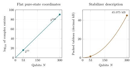
The memory question is equally striking. A flat description of a general pure state of qubits has complex entries. A special, highly structured family of states on those same qubits has a packed description smaller than kB. The difference is structure: one representation lists coordinates, while the other stores rules that generate them. Section 5 explains exactly which states fit the small representation and what its byte count includes.
This paper follows those two questions through a proposed finite record framework. We will open the data structures, follow a measurement, and inspect the settings needed to run the next experiment. The console is a way to make the mathematics visible. We begin with the few quantum ideas needed to read its display.
0 Four quantum ideas for reading the console
A qubit and its state. A classical bit has two values, usually written and . A qubit is a quantum system with two distinguishable reference states, also called and . A photon’s horizontal and vertical polarisations provide an example. The word state means the mathematical description used to predict the results of allowed operations. For a classical coin hidden under a cup, probabilities for heads and tails may be all the description needs. A qubit requires more: how we ask the question can reveal information that those two probabilities leave out.
Superposition. Suppose two preparation procedures both give equal numbers of and results when tested in the reference setting. One procedure randomly prepares or and forgets which. This is a probability mixture. The other prepares a particular superposition: a state with a definite relation between the two alternatives. Apply the same suitable rotation before reading each preparation. The mixture still gives balanced outcomes; this superposition now gives with certainty. They looked identical to the first question and different to the second. That is why a list of reference-setting probabilities is insufficient.
The extra relation is called coherence. Its phase determines how alternatives reinforce or cancel when an operation brings them together, much as the relative timing of waves determines an interference pattern. Saying that a qubit is “both zero and one” is a shorthand; the useful fact for a programmer is that the state must retain enough information to predict these interference effects. One read returns one ordinary result. Repeating the preparation and changing the operation reveals the structure behind the results.
Entanglement. Now prepare two qubits together. The description of the pair can contain information that neither member’s local description contains. In the example below, either detector sees a balanced random sign. Yet suitable comparisons of the two records reveal exact correlations. This alone could happen with classical correlated coins. The quantum distinction is that the correlations across several different measurement settings require a joint state that cannot be assembled as a probability mixture of separate local states. This is entanglement: a property of the pair and its preparation. Each member still has a local state, but the two local states together leave part of the joint description unspecified.
Measurement. A measurement chooses a question, produces an outcome and changes the state available for later operations. The physical apparatus determines which question is asked. Quantum mechanics supplies probabilities for its outcomes and a rule for updating the state after a specified outcome. A program therefore needs both a result and an updated state, just as a stateful method returns a value while changing its object. A saved result can subsequently be copied and compared as classical data. Preparing, reading, retaining a result and resetting the apparatus are separate steps.
Later we use a density matrix to put these ideas in one data structure. Its diagonal entries give the probabilities of the chosen reference labels. Its off-diagonal entries retain coherence, which other operations can turn into changed outcome probabilities. A reduced state is the description sufficient for operations on one member of a larger system. These names will let us say precisely what a console has stored and which queries it can answer.
Scope of the comparison
The reference labels always belong to a specified measurement setting. Coherence can be detected through interference; it is not hidden from every possible observation. The small programs here use the standard quantum probability and state-update rules as supplied definitions.
1 Watching a pair at the console
The console displays three kinds of object: a preparation, the pair’s current quantum state, and the records returned by its two readers. The preparation has an identifier. Each result carries that identifier, a reader name, a measurement setting and an outcome. A comparison process later matches the two results. This is the same practical discipline used in a database: related facts need an explicit key.
For the preparation called the Bell state , each local state is maximally mixed. In plain terms, every projective spin measurement along a specified direction gives balanced local outcomes. The pair’s joint state supplies the correlations. If the console stored only the two local states, it would lose the information that distinguishes this preparation from other preparations with the same local behaviour.
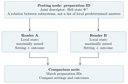
The comparison is a relational join followed by a calculation. Match the preparation identifiers, multiply the two recorded signs, and average those products over repeated trials. An average of means the signs always agree, means they always disagree, and zero means no average sign correlation. The settings , and name three standard, mutually perpendicular quantum measurement directions. For this Bell pair the exact table is:
The minus sign on is a useful test of the implementation. A routine that hands both readers the same random sign would reproduce the row’s agreement and fail on . The joint-state object must contain enough information to answer all the supported questions.
A second comparison shows why coherence matters. Prepare half the time and half the time, then forget which was prepared. This classical mixture has the same local randomness and perfect agreement as the Bell state. Its correlation is zero, whereas the Bell state’s is . A record of the tests alone cannot distinguish the two preparations. Changing the question reveals the difference.
The quantum resource also has a lifetime. In this example, after the first local rank-one projective read, the conditioned pair state becomes a product of its local states. The original entanglement has been consumed. The software retains the updated state for the other reader, together with the preparation identifier and the classical results. A useful resource flag therefore says whether the original Bell preparation remains available. Keeping its identifier is different from keeping that resource available for another experiment.
This answers the opening storage question at the logical level. The pair row holds a descriptor of the joint state; the two result rows hold classical outcomes. Comparing results requires the latter. Predicting another supported read can require the former. A pointer to the descriptor tells the program where to look, while the descriptor’s implementation determines how much memory and calculation it needs.
The mathematical contract for an outcome-bearing call is a quantum instrument, following Davies and Lewis [8]. It specifies outcome probabilities and conditional state changes. A familiar method signature captures the idea: supply the current state and a setting; receive an outcome record and the next state. Appendix A gives the concrete code and its logical systems specification.
Scope of the comparison
The drawing shows logical dependencies in a central program, not physical communication paths. The displayed table is not itself a Bell-inequality violation; the program separately checks the required rotated settings. A classical simulator may copy its known state arrays, while respecting the represented system’s restrictions on broadcasting unknown quantum states [4]. The pair-row analogy makes no claim about a database normal form or a general rule for multipartite entanglement.
2 Wheeler’s question, and the machinery of an answer
Wheeler asked a more ambitious version of the console’s question. His phrase “it from bit” placed questions and registered answers near the foundations of physical reality [42]. It can be read as a programme for reconstructing physics from information, or as a participatory account in which the questions help constitute the world being described. Our systems account takes up the practical machinery that either reading needs.
Wheeler illustrated participation with a variation on twenty questions. The answerers had chosen no word in advance, but each new reply had to remain compatible with the previous replies. The eventual answer depended on the questions and the accumulated constraints. The image directs attention away from an inventory of ready-made answers and towards the process by which a consistent answer becomes available.
A programmer following that image immediately needs an interface. Which questions are legal? Which can be asked together? What changes after an answer? What must be retained for the next call? A random-number generator can choose among supplied alternatives, but someone still has to define the alternatives, their weights and the state update. These are parts of the specification.
Consider a detector with a display marked red and blue. The labels are its output alphabet. Behind that display, the apparatus might be testing polarisation, charge or a temperature threshold. Each implementation has its own coupling to the measured system and its own behaviour when read again. The colour tells us the answer only after we know the question and the procedure that produced it.
The phrase algebra before bit names this ordering. An algebra organises operations and their composition: which questions belong to the apparatus, which transformations act on its state, and how records can be combined. A particular bit is an answer within that organisation. Starting with the algebra lets us specify the spaces in which answers have meaning, then ask what further rules generate and retain them.
Landauer adds the physical memory behind the display [38, 39]. Information has an embodiment. Resetting that memory involves an environment and an accounting of correlations, heat or work. Bennett’s reversible-computation analysis shows why the timing of disposal matters [6]: many computations can retain enough information to be undone, with erasure postponed to a distinct step. Together these ideas encourage a systems description with a data model, an operation model and a resource model.
The constructive task is now concrete. List the possible records, give each operation its inputs and state changes, and say what survives for the next operation. A philosophical question has become a sequence of implementable questions. The finite framework discussed here provides objects with which to begin answering them.
Scope of the comparison
Wheeler’s participatory ambition is broader than this paper’s systems representation. An algebra specifies an organisation of possibilities; the physical apparatus, dynamics and outcome weights require their own account. Landauer’s erasure principle applies under stated thermodynamic conditions, rather than assigning a universal energy cost to every recorded bit.
3 The framework: cells, records and questions
The framework begins with finite registers and quantum error correction [16, 22]. Error correction organises physical degrees of freedom so that specified disturbances can be detected or corrected. For a systems reader, it provides a vocabulary of allowed states, checks on those states and operations with declared input domains. The framework develops these ingredients into an account of records and their interactions.
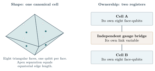
Its characteristic cell is an oblate square bipyramid: two shallow pyramids joined along a square equator. Each of its eight triangular faces carries a qubit. Cells occur in three orientations, with their apex axes aligned along the three perpendicular bond directions. Distinct cells own distinct registers. Their coupling is represented through gauge bridges with independently owned degrees of freedom. Figure 2 separates the cell’s shape from that ownership relation.
Now choose the record labels that an apparatus can distinguish. Each label has a projector, a mathematical test selecting that label’s sector. The projectors for mutually exclusive labels commute: applying those record tests in either order gives the same result. Their linear combinations form the record algebra. It collects the numerical questions answerable by inspecting that particular record.
The density matrix introduced in the primer puts the distinction between label probabilities and coherence on the page. For two reference labels it has the form
Read only the reference labels and the off-diagonal entries leave the displayed probabilities unchanged. Apply an interference operation before reading and those entries can affect the answer. For our two preparations in the primer, the diagonal entries agree while the coherences differ. The state stores the extra information needed by the enlarged set of questions.
An actual record and its probability belong to different levels of the description. On one trial a detector returns a label. Across repeated preparations the state predicts a distribution of labels. The label is the event stored in a result row; the population is a weight used to predict such events. Keeping those levels separate makes the data model easier to read.
The framework offers three useful views of this process [13, 20]. The count view retains totals: reads, commits, exports and service events. Think of a web server’s hit counter. It tells you how many visits occurred, while the request log tells you what the visitors did. Both are useful, but they answer different questions. A performance counter can expose an unexpected operation without retaining enough history to predict the next response.
The record view keeps labels, owners and links between records. Preparation identifiers let us pair two detector results correctly. A stored label can be enough for one calculation and insufficient for another. A summary is sufficient only for the questions it was built to answer.
The response view specifies the query applied to those results. A display might report just “some numbered outcome occurred”, grouping many labels into one bin. Two processes could move probability between those labels while leaving that display unchanged. A query asking whether the same label appeared twice uses information that the coarse display discarded. Choosing an observable is therefore like choosing an aggregate query: it determines which differences become visible.
The Ledger Is Not Enough gives two concrete tests of this distinction [29]. In one fixed repeated-use model, two reachable histories have equal service counts but predict different next-read distributions. The counter alone is insufficient for that prediction. A separate test compares different models that agree on first use and disagree later. That test concerns an incomplete rule for future behaviour. The first is a missing-state problem; the second is a missing-law problem. A systems specification needs a place for both.
The same study finds equal single-read statistics with different two-read correlations. Keeping the relation between successive labels exposes differences that single-use summaries hide. The console can display each level side by side: the counts, the retained records and the query used to turn them into a reported statistic.
Scope of the comparison
The cell illustration uses the canonical bond-centred oblate geometry. A spatial embedding, the disjoint register ownership and a physical propagation law are separate objects. The Bell program is a two-qubit example, not a simulation on that spatial graph. The ledger comparisons are conditional finite-model results; their physical instruments and response maps remain to be identified. Coherence is outside the chosen record algebra, not outside observation altogether.
4 From a console picture to a systems description
A console is most useful when every box has a contract. The pair’s current state, its preparation history and its outcome records have different jobs. A logical data model names those objects and their relationships. A process model says which operation reads or changes each object. A life-history model says which sequences of events are permitted.
For the Bell demonstrator, the life history is short. Create a fresh preparation. Read either endpoint. Read the other. Compare the two records as often as required. The two reads change the quantum state; repeated comparison uses the saved classical records. A second read of an already-used endpoint is outside this example’s contract, so the program rejects it. The system has an explicit answer to what may happen next.
This makes coherence a manageable software concept. It belongs inside a typed QuantumState value, with operations for computing outcome probabilities, updating after a result and extracting a local state. The data model can name that value without prescribing an array, a compressed descriptor or a database field. The process contract supplies the mathematics that the chosen implementation must respect.
The distinction between a type and an implementation is familiar. A set type promises membership, insertion and deletion; its representation could be a list, a tree or a hash table. A quantum-state type promises a more demanding collection of mathematical operations. Its implementation might use a density matrix for a small example and a structured representation for a larger supported family. In both cases the interface must preserve the promised answers.
Appendix A turns the Bell example into a conventional logical systems specification: data dictionary, data-flow diagram, entity life history, event–entity effects and a read-process contract. It uses SSADM and Jackson-style notation from the structured-analysis tradition familiar in the 1980s [3, 33]. These notations are useful here because they make us write down data dependencies and legal event sequences explicitly. The conventions are explained beside the diagrams, so familiarity with those methods is unnecessary.
This fourth, systems view connects the other three. Counts support accounting, records support later comparisons, and responses define the questions being answered. The process model shows when each is needed. For example, the second quantum read needs access to the current state, while the final sign-product comparison needs only two outcome records. The distinction becomes a checkable dependency in a diagram and in code.
Scope of the comparison
Appendix A specifies one central Bell service, including its supplied quantum rules. It is a worked example rather than a full specification of the framework. Logical locations on its diagrams do not assign objects to positions in physical space. A wider implementation must supply its own concurrency, reuse and distribution contracts.
5 Memory: store the structure when structure suffices
Return to the two memory figures on the opening page. A conventional pure-state description of qubits has complex amplitudes. An amplitude is a number used to combine quantum alternatives; its phase matters when alternatives interfere. The flat representation lists one amplitude for each reference configuration. At the count is about ; at it exceeds . These are coordinate counts, before removing normalisation and an irrelevant overall phase.
A stabilizer state takes a different route. It is specified by a set of quantum constraints that generate its structure. A stabilizer is an operator that leaves the state unchanged. Instead of listing the enormous set of amplitudes, the program stores a compact set of those constraints. This is generator form: give the rules needed to recover the structure, then calculate the requested property from them.
The advantage extends beyond storage. Gates in the Clifford family carry the relevant Pauli constraints into other Pauli constraints. The description can therefore be updated directly, and suitable Pauli measurements can be evaluated efficiently. Gottesman’s account and the Aaronson–Gottesman algorithms establish this classical simulation method [1, 35]. A large entangled state can be easy for this method when its structure remains in the supported family.
One standard Aaronson–Gottesman tableau stores stabilizer and auxiliary rows, including their signs, in packed bits. At qubits that gives bits, or bytes: below decimal kilobytes. That is the packed state tableau. Instructions, identifiers, buffers and the programming-language runtime add their own memory. Figure 3 keeps the coordinate count and packed storage in separate panels with separate units.
The framework’s executable record grammar uses this distinction to organise a calculation [17]. It keeps record data, stabilizer structure and further phase-sensitive information in separately described parts. Its finite compression certificate asks which observables survive a proposed record projection, and bounds a residual for observables outside that projection. For a programmer, this is a contract for compression: these queries remain exact, while those require additional information or an error allowance.
The extra resource beyond stabilizer methods is often called magic. The name refers to states or operations outside the efficiently handled stabilizer subtheory. Such operations can make a compact simulation much more expensive. The useful question is how much of this resource the allowed computation introduces, how it composes and what the requested observable requires the program to retain.
A holonomy register is one way to organise phase-sensitive information associated with closed paths. Think of carrying an internal orientation around a loop and comparing it with the orientation at departure. The loop records the accumulated transformation. Giving that information a named place in the state description lets the program track its cost and its effect on observations.
This gives the console a practical response when the next operation exceeds its present representation. It can enlarge the state object, switch algorithms, approximate under a declared error bound or reject the request. The choice is part of the implementation contract. A compressed object that answers all fixed record questions may be useful even when a later interference experiment needs a richer description.
The benchmark must count evaluation as well as storage. A short file can encode a calculation that takes a long time to run. Requested accuracy, circuit connectivity, entanglement structure and the distinction between sampling an outcome and calculating a tiny probability can all affect the cost. The console should display the supported query family alongside the memory use, so the resource claim travels with the operation it supports.
Scope of the comparison
The small tableau applies to stabilizer structure and the specified operations. It is not a general bound on a quantum universe simulator. A phase or holonomy register must also have a controlled size and evaluation cost. The framework’s finite certificate supplies a checked starting example; resource growth under wider composition remains a research question.
6 Brokers, grammars and compilers
An interaction vertex can be read as a broker: it accepts particular inputs and produces particular outputs. Its type signature includes charge and representation labels. A proposed interaction passes only if those attributes fit the rules. This resembles checking an API call against its schema, with conservation constraints doing part of the checking.
The broker also carries an amplitude weight. Here quantum arithmetic changes the software picture. Alternative interaction histories can reinforce or cancel, so the program combines their complex amplitudes before obtaining probabilities. Sampling one diagram at a time with ordinary traffic-rate weights would generally lose that interference. The type system organises the possibilities; the amplitude calculation determines their combined response.
The framework develops this compiler reading in its attribute-grammar account of the Standard Model [25]. An attribute grammar attaches properties to symbols and propagates them through permitted productions. Here the attributes include representation and charge information. A successful derivation tree records how the proposed interaction satisfies the supplied rules, making its consistency inspectable.
The semiring formulation separates the grammar from its arithmetic [24, 34]. The same structure of derivations can answer different questions: does any legal derivation exist, how many exist, or what is their combined amplitude? Each task uses its own rules for combining alternatives and composing steps. “Semiring” names that algebra of combination. Its engineering value is the possibility of reusing common subcalculations while keeping the meaning of their arithmetic explicit.
The qgrammar project provides a corresponding front end [19]. It handles typed matter data, rule checks and output scaffolding for a larger physics workflow. Checking an interaction vocabulary, testing declared anomaly conditions and generating input for another tool are concrete software jobs. The compiler makes the assumptions visible at the point where they enter the calculation.
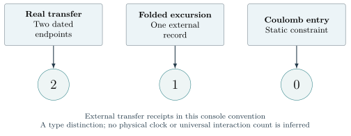
The schematic gives another use of types. In the framework’s conditional transfer classification, a real transfer has two dated external endpoints. A folded virtual excursion has one external record. The Coulomb entry is a static constraint or debt contribution, with zero propagating-transfer receipts in this convention. The diagram counts external transfer receipts; that is the field represented by the three numbers.
The word “external” is relative to the enclosing operation. Information retained inside a carrier and a record exported from it have different roles in the accounting. A static field can affect a detector while contributing zero to this particular propagating-receipt count. A folded excursion can contribute its one external record while lacking the two dated endpoints used for the real-transfer category. Appendix B identifies the source and scope of this rendering.
Shared computation is also useful for sums over histories. A program can store common prefixes or subexpressions once and accumulate their weights through a graph of alternatives. It need not create a separate host process for every history. This is the same economy that makes compilers and dynamic programming useful, now applied with quantum amplitudes and their interference intact.
Scope of the comparison
The compiler validates supplied assignments and organises calculations; deriving their physical values is a further task. The convention is not a general definition of real and virtual particles, and it selects no proper-time law. Shared subcalculations provide an implementation technique, not a general polynomial-cost bound for interacting amplitudes or an interpretation of quantum branches.
7 Measurement as a commit protocol
Follow one invocation through the console. It begins with a current state and a chosen question. It ends with an outcome, a new state and a decision about the stored record. Separating those stages gives “measurement” the detail that a stateful software interface requires.
First comes the monitor: the physical coupling that makes a question accessible. A detector reading polarisation needs an interaction sensitive to the selected polarisation distinction. The framework’s pointer-selection analysis distinguishes the candidate record states from the mechanism that reads them [18]. The console can attach a source and a status to that monitor, just as it does to other supplied components.
Next, subject and apparatus can become correlated through reversible premeasurement. If the relevant joint information is retained, this step can in principle be undone. Selecting an outcome, retaining it as a readable record and preparing the apparatus for another use are subsequent operations. The framework’s treatment of transitions and records uses instruments and export conditions to specify those boundaries [26].
The probability step uses a weighting rule. The usual Born rule converts amplitudes into predicted outcome frequencies. Gleason’s theorem relates such probabilities to the quantum state under assumptions about additive assignments to projectors [32]. The framework studies both a record-sector route and a closed-record-pair calculation [11]. The latter obtains a quadratic diagonal structure from its declared forward/backward pairing. The Bell example simply supplies the ordinary Born rule, so readers can inspect the state and record bookkeeping directly.
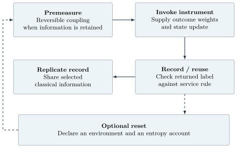
A commit writes the result according to the service convention. The current occupied-cell rule performs a read on every invocation and counts a new commit and service bill when the returned label differs from the previous label. On the original blank-input domain it reproduces the first-use counts. Thus the read count and the changed-label write count answer different accounting questions.
Reusing the apparatus makes the retained state important. Imagine two successful calls that leave the display showing the same label. They might leave different joint states of the measured system and apparatus, so a later operation could distinguish them. By contrast, an isolated rank-one pointer read fixes its local state once the label is known. The carrier tells us which case is being described. The ledger study tests this distinction explicitly [29].
Eventually a memory may be reset. For an unbiased classical bit erased isothermally without using side information, Landauer’s ideal minimum dissipated heat is about electronvolts at kelvin [38]. This example gives the reset a physical resource account. A practical device also needs its actual input distribution, correlations, implementation losses and available work resources included in that account.
The software image of garbage collection helps locate one part of this process: an operation makes information unavailable to the subsystem whose future we track. The physical account follows where that information or its correlations went. Reversible preparation, readable output and irreversible disposal can then be distinguished in the event log and in the thermodynamic model.
A durable outcome may finally be replicated. Quantum Darwinism examines how multiple environmental fragments acquire accessible information about selected observables [44]. The framework’s syndrome-broadcast construction gives a conditional error-correcting version of that idea [14]. Several readers can recover compatible record information from different fragments. This is the step that turns one apparatus result into a widely available fact.
Scope of the comparison
The commit convention is a conditional service rule, not a universal dissipation law. Landauer’s number belongs to the stated erasure setting. The garbage-collection image does not derive the Born rule or explain a unique experienced outcome. Gleason’s standard theorem has a dimension restriction; the closed-pair calculation has its own assumptions. Replicated record information is distinct from unrestricted copying of an unknown quantum state.
8 Nonlocality and the price of a clock
The Bell console illustrates two facts at once. Joint records can exhibit correlations stronger than local response rules permit under Bell’s locality and statistical-independence assumptions [5]. Yet each reader’s local distribution can remain unchanged when the other reader changes setting. Correlation and signalling are different operational questions, and the program checks them separately.
The comparison node estimates correlations after receiving the classical records. It obtains useful information by matching the two results, just as the original console picture suggested. The joint-state descriptor is what allowed the program to calculate the quantum distribution in the first place. A small descriptor can therefore represent correlations that local marginal descriptions leave unspecified.
Experiments such as Hensen and colleagues’ separated-spin test make the physical question concrete [36]. Any proposed account of how nature produces these correlations must meet the experimental constraints. The central Bell program supplies the standard quantum calculation as a reference against which such accounts can be tested. Its internal organisation is visible to us because we wrote it.
That visibility exposes the clock question. An ordinary simulator processes instructions in a host order. Its event queue might choose one reader first for convenience. If both allowed orders give the required operational predictions, that implementation choice can remain part of the software. The situation changes if a theory identifies the queue with a universal physical tick. It has then added temporal structure to the physical model.
A universal physical ordering would need an account of moving observers, clock comparisons and observable covariance. Round-trip messages can define clock readings, but the model must also establish how the messages and clocks behave. The propagation-clock and relativity papers offer conditional targets for this work [21]. The console’s clock setting makes the remaining choice easy to locate.
Loop variables fit naturally into the data model. A holonomy stores the transformation accumulated around a closed path; its value can be present in a state description before a reader asks about it. To turn that object into a physical mechanism, the model must specify how it is prepared, changed and measured. The same discipline used for the Bell instrument applies to the loop variable.
Gravity adds a relation between matter, geometry and the quantities available to instruments. The gravity–measurement seam analysis separates those components [28]. A systems account can show which source rule feeds which geometrical construction, and which map connects that construction to an observable. This is useful dependency information for the next calculation.
Scope of the comparison
A joint descriptor represents quantum correlations; it does not evade Bell’s theorem or supply a communication mechanism. Host scheduling is a physical preferred-frame commitment only if identified with physical time. The historical Lorentz calculation on a superseded lattice is not evidence for the current canonical geometry. Recovering relativistic dynamics and a gravitational endpoint remains separate work.
9 The unresolved settings are the test
Open the console’s settings panel. Some entries are defined by the example; others remain choices in the framework. Leaving those entries visible is productive. It tells the programmer what must be supplied for a run and tells the physicist which changes might alter its predictions [23, 29].
Six headings provide a practical inventory. History weights determine how alternative histories contribute to a result. The clock connects an ordering or count to a physical time variable. A carrier map translates between mathematical descriptions so that an endpoint question has the required input. Re-entry specifies what happens when an occupied system is invoked again. The schedule orders or coordinates the invocations. A pair service unit specifies the weighting used when a statistic bills pairs of events.
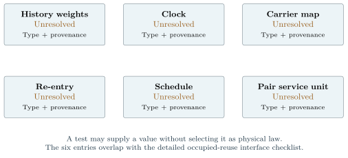
Each setting has a type. A carrier map might translate a probability distribution, pull an observable back to another description, or perform another declared operation. A clock setting needs units and a calibration; a schedule needs an ordering rule. Calling them all numerical parameters would obscure the interfaces between them. A useful console shows a type, a source and a status for each entry.
A finite review of occupied reuse provides a more detailed checklist. Its frozen sources left eleven required fields unspecified: the retained-information carrier; the read instrument; reset; allowed controls; the schedule; identification between the compared carriers; the first candidate’s extension to occupied inputs; the second candidate’s extension; re-entry selection; the endpoint carrier map; and the selected physical reuse law. These are the fields an implementation needs before it can execute that particular comparison as a unique test.
The six console headings and eleven interface fields overlap. They describe the same gaps at different levels of detail. A broad heading such as re-entry can expand into several interface requirements. Later work may derive a field, identify it with an existing object or replace the interface with a better formulation. The checklist records what is currently missing from the specified comparison.
An executable premise ledger gives each input a provenance record: where it came from, its status, the carrier on which it acts and the uses it permits. A derived entry points to its assumptions and verifier. A supplied entry remains labelled in the output. An unresolved entry prompts the caller to choose a supported family of tests or supply the missing input. The framework’s canon and verification methodology implement this discipline [10, 12, 27].
A family of candidates already supports useful experiments. Hold the other inputs fixed, vary one admissible choice and measure the same observable. A change in the result identifies freedom the observation can detect. An unchanged result may identify an insensitive query or a genuine invariant across that family. Both outcomes help determine what a future physical principle needs to select.
The same logic tests a proposed principle. If it accepts every candidate, it makes no selection within the family. If it accepts none, it exposes an incompatibility. If it excludes some and retains others, the excluded alternative is the witness of its selective force. A result becomes persuasive through that comparison, rather than through the appearance of one favoured example.
Dependencies also determine which research can proceed. The correction and coherence construction can advance on its declared mathematical inputs while an occupied-reuse interface remains open, provided its hypotheses do not use that interface. The physical origin of an inner product or a clock enters where the construction actually requires it. The systems account keeps these dependencies visible instead of treating every open problem as a block on every other one.
Scope of the comparison
The six headings and eleven fields are overlapping inventories, not seventeen adopted axioms. A replay checks a computation under its declarations; empirical identification needs further evidence. When a result is exported, its supplied weights, clock calibration and response map must travel with it. This preserves the distinction between a family of conditional predictions and a selected physical law.
10 Can the console run on a classical computer?
For the stabilizer fragment, the answer is yes under the operations described in Section 5. For extensions, the cost depends on the state family, permitted operations, requested observables and accuracy. The record-grammar certificate retains a place for additional phase-sensitive information [17]. Measuring how that part grows under composition is the next resource question.
The -qubit superconducting experiment of 2019 shows why the task matters. Arute and colleagues compared a random-circuit sampling experiment with the classical methods considered at the time [2]. Subsequent classical simulation work revised the practical comparison [37]. The number of qubits identifies the size of the carrier; the circuit family, sampling task and algorithm determine the computational contest.
A useful benchmark for this framework would begin with an increasing family of valid preparations and operations. It would state the observables, accuracy, time and memory required, and track the part of the cost associated with non-stabilizer information. Include sequences that accumulate that information as well as examples that preserve simple structure. Count the input description and observable evaluation alongside the stored state.
One possible result is a proved restriction keeping a relevant resource small enough for a specified classical algorithm on the physically allowed family. Such a restriction would be a substantive physical and computational proposal. Its excluded processes would give experiments something to test. Another result is that the accessible record layer stays compact while its quantum state remains expensive to simulate classically. A quantum implementation could then carry that state, with ordinary software managing settings and records.
Controlled approximations and restricted query sets offer further useful outcomes. A simulator might handle an important class of observations with an explicit error bound while declining other requests. A description might save memory but require expensive evaluation. These are measurable properties of an implementation, and the console can report them in terms a systems reader recognises.
The first benchmark should start small. Reproduce the finite certificate, compose supported operations, track the retained objects and identify the first query requiring a more expensive representation. On small carriers compare the compact calculation with direct matrix evolution using the same preparation, instrument and observable. Deliberately submit incompatible queries to check that the interface catches them. Larger cases then have a measured baseline and an explicit account of what has been proved, checked numerically or extrapolated.
Scope of the comparison
A small demonstration or a large amplitude count settles neither general classical feasibility nor general hardness. The decisive resource bound for the framework’s wider allowed dynamics remains open. The bedroom-computer image supplies a question about implementation cost, not a prediction that the cost will be small.
11 How this relates to other computational pictures
Several approaches connect information and physics. The useful comparison is what each aims to explain: physical dynamics, the interpretation of quantum theory, or the requirements of a computational representation.
Bostrom’s simulation argument concerns populations of observers and ancestor simulations, conditional on assumptions about technology, choices and observer counting [7]. Our console instead asks what data and operations represent a finite quantum framework. It assigns no probability that we inhabit a simulation.
Fredkin’s digital philosophy places discrete informational dynamics near the foundations of physics [31]. Wolfram investigates the elaborate behaviour obtainable from simple computational rules [43]. Here the starting point is an explicitly quantum carrier, a record algebra and declared operations. We examine their interfaces and implementation costs.
’t Hooft seeks a deterministic underlying description and its relation to quantum states [41]. Our Bell routine supplies ordinary quantum probabilities. Its pseudorandom seed makes a transcript reproducible; a physical deterministic account would separately have to specify its locality, independence and other assumptions.
Lloyd’s account of the universe as quantum computation is a close neighbour [40]. Our emphasis is the accessible record layer: the questions it answers, the information its summaries omit and the inputs connecting it to observations.
Everett’s relative-state formulation addresses the interpretation of unitary quantum mechanics [30]. A simulator’s graph of alternative derivations organises a calculation. Sharing subexpressions saves work while preserving amplitudes; identifying alternatives as physical worlds is a separate question. Deutsch’s universal quantum-computer analysis concerns possible computational implementations [9], which can be discussed alongside different interpretations.
Scope of the comparison
The console adopts no simulation probability, hidden-variable interpretation or many-worlds ontology. A universal physical scheduler would still need the covariance account discussed in Section 8. The contribution here is an inspectable specification: it gives the next physical construction a named interface to complete.
12 The first program to run
Return to the console and its pair of apparently random records. We now know which object holds the joint description, which data each reader returns and which comparison reveals the correlation. We also know why a small counter can lose predictive information, why a quantum state needs coherence, and why a compact description must be assessed together with its supported operations.
The first program is already supplied. Prepare the Bell pair, display its two local states, select the measurement settings, store the outcomes and join them by preparation identifier. Check the exact correlation table before sampling it. Check no-signalling separately. Retain the updated state for the remaining reader and retire the original entangled resource after the first local projective read. Appendix A shows the implementation and the systems contracts it follows.
The next experiment is composition. Which information does the next call need? Which queries survive a record projection? Which supplied settings change the observations? How do memory and evaluation time grow? These questions connect the framework’s mathematical structure to work that can be performed and measured. A successful derivation can replace an open setting; surviving alternatives can remain visible as a family to investigate.
This is a representation, not a hypothesis: nothing here says the universe is a simulation, and nothing here depends on it being one. Putting algebra before bit gives the recorded answer a place in a larger specification. That specification is the paper’s practical contribution: a way to follow the data, run a small example and see exactly what the next piece of physics must provide.
Data, code, and source status
The companion directory contains the reference program, numerical verifier, claim index, and a source manifest. Its authorial checks cover the declared examples and source bindings. Published framework sources are cited by version DOI; the recent reuse-interface result is bound separately in the source manifest. This preprint is archived at doi:10.5281/zenodo.22650176. The bibliography records primary-source metadata checked on 7 September 2026. The accessibility revision preserves the original Bell calculations, Appendix A and bibliography. Its additional figure is reconstructed from authenticated canonical geometry sources.
Acknowledgement of assistance
The author used OpenAI Codex to assist with drafting, source checking, programming, and typesetting. Responsibility for the claims and any submission rests with the author.
A A worked systems specification: the Bell demonstrator
A.1 Boundary, purpose, and supplied rules
The following is a small logical systems specification of the reference Bell demonstrator. It uses the data, process, and entity-life-history views familiar from SSADM, with the notation stated alongside the diagrams [3, 33]. It is a tailored worked example, rather than a claim to have completed every stage of that methodology. Its purpose is to make the explanation checkable against an existing program.
The boundary encloses a single-process Bell experiment service. Its external actor is the experiment driver, which requests a preparation, requests local reads, and asks for a comparison. “External” here means outside the selected software boundary. It does not introduce an observer outside the physical universe. The driver supplies fresh preparation identifiers and a pseudorandom draw provider. The service returns a preparation handle, outcome records, comparison results, or errors. The command-line driver is one implementation of that actor; the local readers are roles within the represented experiment.
The fixed profile supplies the Bell preparation, the allowed measurement operators, the Born weighting rule, and the projective state update. Those definitions are constants of this example, not adjustable physical laws derived by the systems analysis. The scope allows one read per endpoint per preparation, in either endpoint order. It excludes reset, occupied-cell re-entry, service billing, spatial propagation, and concurrent requests. The original driver uses a particular sequence within that permitted behaviour.
The primary requirements are: preserve the declared quantum probabilities; associate every returned record with its preparation and reader; prevent a second read of the same endpoint in this fixture; retain the current joint state for the remaining read; and compare only records with the same preparation identity and different readers. An error in a read’s structural preconditions must be detected before the carrier is changed. Numerical invariant failure aborts the calculation; this small program makes no recovery or transactional-rollback promise for such a failure.
A.2 Logical data structure and data dictionary
Figure A.1 separates the lifetime of an experiment instance from its current mathematical state and its accumulated classical records. Entity boxes and explicit cardinalities describe a logical data structure. They do not prescribe database tables, persistent storage, or a location in physical space. A comparison is a derived response, so it is shown separately from the stored entities.
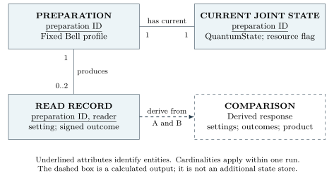
| Entity or value type | Identifier, attributes, and constraints |
|---|---|
| Preparation | Key: preparation identifier, unique within the driver’s run. Created under the fixed Bell profile. It owns the current state and the endpoint read records. |
| Current joint state | Key: its preparation identifier. Attributes: a QuantumState value and the flag indicating availability of the original entangled resource. Exactly one current state per live preparation. No historical versions are implied. |
| Read record | Composite key: preparation identifier and reader role. Reader is A or B; setting is a declared operator name; outcome is a sign. There are zero, one, or two records per preparation, with no repeated reader key. |
| Comparison response | Derived from two read records of the same preparation, one from each reader. Contains the preparation identifier, the settings and outcomes in operand order, and their sign product. It introduces no new quantum state. |
QuantumState |
An abstract mathematical data type. Here its concrete representation is a complex matrix on the declared two-qubit carrier, Hermitian, positive and of unit trace. Its entries include coherence in the declared basis. A handle to it is not an independently readable physical record of all those entries. |
The permitted operations on QuantumState include preparing the fixed state, calculating local outcome weights, conditioning on a selected local outcome, and calculating a reduced state. Coherence belongs inside this structured value, together with the populations with which its consistency conditions are coupled. It is not an independent collection of freely editable facts. In a program, these operations can be implemented as functions or methods; at the logical level their contracts specify the required behaviour without prescribing either choice.
For this small example, preparation identity and the current payload live in one Python Pair object. The logical separation does not require another allocation or a database join at every read. Conversely, combining fields in one object does not make the concepts identical. The resource-availability flag describes the original Bell resource; it is not a declaration that all correlations or all stored data disappear when the flag becomes false.
A.3 Data flows and elementary processes
Figure A.2 decomposes the service into numbered processes. Arrows carry named data, not elapsed time or physical signals. Open-ended stores identify retained information; the closed rectangle is an external actor. The context-level inputs and outputs listed above are preserved by the decomposition. The immutable quantum profile is part of the process definitions, rather than an unlabelled runtime input.
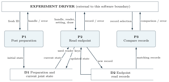
Process P1 creates the preparation and initial joint state. P2 reads the current state and the already-used reader keys, applies the declared instrument, updates the current state, and adds the returned record. P3 reads a matching pair of records and produces a comparison. The implementation passes copies returned by P2 to P3, rather than issuing a database query. The logical read from the record store denotes that dependency, not a particular storage mechanism.
This decomposition makes an important requirement visible. P2 requires the joint-state payload as well as the record store. Its second invocation cannot be specified from the first record alone unless a separate sufficiency result permits that reduction on the declared carrier. P3, in contrast, can calculate its sign product entirely from classical records. The two processes therefore have different information requirements even though both eventually return ordinary numerical data.
A.4 Entity life history and event effects
The preparation’s life history is shown in Figure A.3. It uses a Jackson-style hierarchy: children are sequenced left to right; circles mark alternative branches; an asterisk marks repetition. It describes completed trials. An unfinished trial may be a prefix of the history, and an error aborts the current request or run as specified below. Both endpoint orders are legal; comparison may be repeated without changing the carrier.
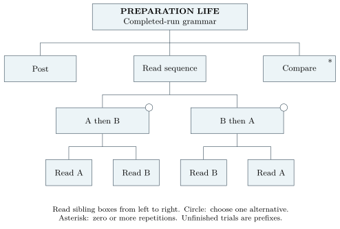
The related read-record history is simpler: it is created by its successful endpoint read, may be consulted by comparisons, and is not updated by this example. The current joint state is created by posting and transformed by each successful read. These views meet in Table A.2, a compact event–entity effect matrix. It plays the cross-checking role of an effect-correspondence model without adding another large diagram.
| Event | Preparation | State | Records | Response | Meaning |
|---|---|---|---|---|---|
| Post | C | C | – | E | Create a fresh experiment instance. |
| Read A or B succeeds | R | R/U | R/C | E | Check reader uniqueness; condition the state; retain one new record. |
| Compare | R | – | R | E | Read the two genuine records and return their product. |
| Structural request rejected | R | – | R | E | Return an error; no state or record update. |
After posting there are no read records and the original entangled resource is available. After either first local projective read, one record exists and that resource is consumed. After the other endpoint is read, both records exist and comparison is enabled. The current joint state still exists in both latter cases. Its destruction is not part of this logical service, and a repeated comparison does not consume another quantum resource.
A.5 Process specification P2: read one endpoint
The following contract is the part of a systems description that a diagram cannot replace. “Apply the instrument” is expanded into a defined mathematical operation, while its physical adoption remains a supplied premise of the fixture.
Inputs and preconditions. A live preparation, a reader role, a setting from the fixed profile, and a draw provider returning a number in the unit interval below one. The reader has no existing record for this preparation. The current payload is a valid state on the declared carrier. Preparation identifiers and genuine record provenance are maintained by the caller within the run.
Calculate outcome weights. Obtain the two projectors for the requested setting, acting on the requested subsystem and as identity on the other. The weight of each sign is the trace of the current state with the corresponding local projector. These are Born weights supplied by the profile; they are nonnegative and sum to one.
Select and condition. Use the draw to select a sign according to those weights. Multiply the current state on both sides by that outcome’s projector and divide by its nonzero weight. The result is the conditioned joint state, not merely a new display label.
Successful effects. Store that state; mark the original Bell resource unavailable; add the record keyed by preparation and reader; return a copy of the record. The other reader’s existing record, if any, is preserved. Postconditions include normalisation and the product-state property appropriate to this rank-one local read of the fixture. The program checks the latter at runtime; the companion verifier checks both.
Rejections and limits. Unknown settings, invalid reader roles and already-used readers are rejected before the payload is assigned. A numerical invariant failure aborts the calculation and does not promise rollback. P2 defines no occupied-cell reset, re-entry, physical service charge, or spatial signal.
P3’s contract is deliberately shorter: accept two genuine records produced by this run, require the same preparation identifier and different reader roles, and return the sign product together with the input labels and settings. It does not call a quantum-state method or mutate stored records. Matching text identifiers alone cannot establish provenance for arbitrary caller-created records. The closed driver meets the genuine-record precondition; the exported helper is not a general record-authentication service.
A.6 Implementation correspondence and checks
The diagram and dictionary names are logical names. P1 corresponds to Pair(...); P2 to Pair.read; P3 to join. The current-state store maps to Pair.rho and its resource flag. Read records map to Pair.records and the returned copies. Preparation identity maps to Pair.pair_id. The profile maps to the fixed preparation and setting definitions. This correspondence specifies what can be checked, without claiming that the implementation has a persistence layer or a generic service interface.
The additional verifier, verify_bell_systems_spec.py, exercises both read orders, every declared pair of settings, and every supported outcome branch. It checks the event effects, reader-key constraint, conditioned-state invariants, preservation of records under comparison, and early rejection of invalid requests. It also checks that the logical life-history transitions and process/store dependencies declared in the machine-readable specification agree with the reachable operations. The ordinary paper verifier continues to check the quantum correlations and source bindings.
Two boundaries remain visible. Global preparation-ID uniqueness is a responsibility of the shipped driver; constructing separate Pair objects with the same text identifier is not rejected by the helper class. Likewise, the comparison helper does not authenticate arbitrary supplied dictionaries. Those are explicit preconditions of this bounded, in-process example. A larger service would have to enforce them at its boundary. No new quantum assumption is required to identify either requirement.
A.7 Where occupied reuse would extend the specification
The Bell example has a complete supplied instrument but no occupied-cell service ledger. Extending it to the framework’s reuse question would require the retained carrier, read and reset operations, controls, schedule, carrier identifications, candidate extensions, re-entry choice, endpoint map, and law identified in Section 9. These are missing process and interface definitions on the frozen perimeter, not omissions that an analyst should fill with defaults.
Even before those definitions are supplied, the declared changed-label rule can be written as an effect constraint: every invocation increments the read count; a changed label also increments the commit and service-bill counts; an unchanged label increments neither of the latter. The carrier transition remains separately specified in both cases. An implementation may also write an audit-log entry on every invocation, but that entry is not thereby a physical commit or an erasure. The data model, event model, and quantum process contract must agree on these distinct effects.
The value of the systems description is this explicit separation. A coherence-bearing state can be a structured data value with well-defined methods. The analysis then establishes where that value is needed, which processes may change it, and which classical outputs they produce. It does not replace the mathematics inside those methods or derive a physical instrument from their signatures.
A.8 Running the reference program
The file supplement/bell_console.py implements the central reference example. It uses Python and NumPy, with no network access and no framework runtime. Its named posting node, readers, and comparison node are logical roles in one process. The program is a new explanatory fixture; it is not a banked physical implementation or a distributed communication protocol.
Related executable work is already public: the framework’s Bell-pair calculation, record-compression certificate, and premeasurement and reset example. Their repository counterparts are hash-bound in the source manifest. These programs provide small reproducible calculations supporting the explanation; none is a simulation of a solar system or a complete physical universe.
The supplied preparation is the Bell state . The supplied measurement rule is the Born rule with local rank-one projective updates. The reader settings are the Pauli axes, with rotated settings added for the CHSH check. “Weights” in the log means these supplied Born outcome weights; it does not select the framework’s open history-weight measure. A seeded pseudorandom generator makes the example transcript repeatable without making its seed a physical premise.
post(pair_id, declared_Bell_state)
verify(local_states_are_maximally_mixed)
verify(exact_joint_probabilities_and_correlations)
verify(unread_remote_measurement_does_not_signal)
for each prepared trial:
    A = read_local(setting_A, Born_rule, update_state)
    mark_original_entangled_resource_consumed()
    B = read_local(setting_B, Born_rule, update_state)
    compare(join_on_preparation_id(A, B))
log(weights="supplied, not derived")
Run from the paper directory:
python3 -B supplement/bell_console.py --seed 20260907
python3 -B supplement/verify_algebra_before_bit.py
python3 -B supplement/verify_bell_systems_spec.py
The first command emits JSON containing exact-table numerical evaluations and a sampled transcript. The expected correlation matrix has diagonal entries and zero off-diagonal entries. The rotated-setting CHSH expression evaluates to , approximately . Each single-reader outcome has probability one half. These are deterministic assertions about the declared matrices; finite sampled frequencies are not required to equal them exactly.
No-signalling is tested both through the joint probability marginals and through the reduced state after an unread remote projective measurement. After a selected local rank-one read, the code verifies that the joint state equals the product of its reduced states. This check licenses retiring the original entangled resource in this example. It does not remove the stored preparation history or erase classical outcome correlations.
The verifier also checks the resource arithmetic and Landauer example. In its tableau convention, the bit count is ; dividing by eight gives bytes and dividing again by one thousand gives decimal kilobytes. The Landauer calculation uses , the exact SI Boltzmann constant and elementary charge, and the stated temperature. It is a conditional minimum, not a simulated heat measurement.
Source bindings are checked separately from these mathematical assertions. The package includes small extracted provenance records, the corresponding full-source hashes and git blob identifiers, and publisher/deposit metadata. With an optional --repo argument the verifier also authenticates the frozen source files from the recorded git commit. The portable run needs only the package and NumPy. Replaying it verifies this explanatory fixture, not the full framework or the thermodynamic and relativistic claims of other papers.
B A translation table and its boundaries
| Framework object | Systems representation | Technical source and limit of the translation |
|---|---|---|
| Framework object | Systems representation | Technical source and limit of the translation |
| Cell and carrier | Owned register; typed interfaces | Foundations and Methodology [16]. Canonical disjoint cube registers and gauge bridges must be distinguished from an embedding used for geometric calculations. A database node does not choose spatial adjacency. |
| Record algebra | Legal record questions and labels | It from Bit, Rung by Rung [22]; Records Say What Can Be Known [15]. Populations are weights over labels, not individual registered bits. The physical monitor still needs identification. |
| Coherence | Retained phase-sensitive information | Records and Responses [20]. Invisibility is relative to specified diagonal observables and instrument hypotheses. It is not a universal permission to discard coherence. |
| Counts and response | Counters and an explicit query | From Counts to Observables [13]; The Ledger Is Not Enough [29]. Equal counts need not fix a future; equal marginals need not fix a joint table. Carrier and law remain explicit. |
| Joint quantum resource | Descriptor linked to both readers | An Executable Record Grammar [17]. A relation can encode correlations compactly in a finite fixture; storage and evaluation costs under general composition are not thereby bounded. |
| Transfer record typing | External receipt arity | The conditional real/virtual/Coulomb source extract in source_extracts.json. Its rendering is a console convention, with the static entry representing no propagating-transfer receipts. It selects no proper-time law. |
| Vertex and amplitude | Typed broker and weighted production | The Standard Model as a Certified Attribute Grammar [25]; Semiring Parsing the S-Matrix [24]; qgrammar [19]. Compiling supplied assignments is not deriving their physical values. |
| Instrument and commit | Outcome-bearing call and service rule | When Does a Quantum Transition Become a Record? [26]; Pointer States Are Not Enough [18]; occupied-cell source extract. A read, changed-label commit, reset, and physical dissipation are distinct. |
| Probability assignment | Declared weighting step | The Born Rule as a Closed Record Pair [11]. Additivity/refinement assumptions and the closed-pair quadratic form have different logical roles. The reference fixture supplies standard Born probabilities. |
| Redundant record | Replicated readable data | Quantum Darwinism as Noisy Syndrome Broadcast [14]. A conditional account of record accessibility, not unrestricted quantum-state cloning. |
| Clock and geometry | Event ordering plus a proposed calibration | Special and General Relativity from the Finite-QEC Substrate [21]; Described Twice? [28]. Implementation order is not yet physical time, and a record correlation is not a spatial metric. |
| Unselected inputs | Settings with provenance and scope | A Physics Canon as a Replayable Algebraic Object [12]; Relocating Trust to the Verifier [27]; Adversarial Self-Registration [10]; A Selection-Rule Calculus [23]. A successful replay preserves conditional status; it does not promote a premise to a law. |
References
- Scott Aaronson and Daniel Gottesman. Improved simulation of stabilizer circuits. Physical Review A, 70 (5): 052328, 2004. doi:10.1103/physreva.70.052328.
- Frank Arute, Kunal Arya, Ryan Babbush, Dave Bacon, Joseph C. Bardin, Rami Barends, et al. Quantum supremacy using a programmable superconducting processor. Nature, 574 (7779): 505–510, 2019. doi:10.1038/s41586-019-1666-5.
- Caroline M. Ashworth. Structured systems analysis and design method (SSADM). In The Software Life Cycle, pages 168–188. Butterworth-Heinemann, 1990. doi:10.1016/B978-0-408-03741-9.50014-3. URL https://doi.org/10.1016/B978-0-408-03741-9.50014-3.
- Howard Barnum, Carlton M. Caves, Christopher A. Fuchs, Richard Jozsa, and Benjamin Schumacher. Noncommuting Mixed States Cannot Be Broadcast. Physical Review Letters, 76 (15): 2818–2821, 1996. doi:10.1103/physrevlett.76.2818.
- J. S. Bell. On the Einstein Podolsky Rosen paradox. Physics Physique Fizika, 1 (3): 195–200, 1964. doi:10.1103/physicsphysiquefizika.1.195.
- Charles H. Bennett. The thermodynamics of computation—a review. International Journal of Theoretical Physics, 21 (12): 905–940, 1982. doi:10.1007/bf02084158.
- Nick Bostrom. Are You Living in a Computer Simulation? The Philosophical Quarterly, 53 (211): 243–255, 2003. doi:10.1111/1467-9213.00309.
- E. B. Davies and J. T. Lewis. An operational approach to quantum probability. Communications in Mathematical Physics, 17 (3): 239–260, 1970. doi:10.1007/bf01647093.
- David Deutsch. Quantum theory, the Church–Turing principle and the universal quantum computer. Proceedings of the Royal Society of London. A. Mathematical and Physical Sciences, 400 (1818): 97–117, 1985. doi:10.1098/rspa.1985.0070.
- David Elliman. Adversarial Self-Registration: A Working Protocol for Keeping a Machine-Assisted Theory Programme Honest. Zenodo preprint, 2026. URL https://doi.org/10.5281/zenodo.21219212.
- David Elliman. The Born Rule as a Closed Record Pair: Measurement, Objectivity, and the Arrow of Time in a Quantum-Error-Correcting Substrate. Zenodo preprint, 2026. URL https://doi.org/10.5281/zenodo.22177177.
- David Elliman. A Physics Canon as a Replayable Algebraic Object: Verifier-Governed Extraction, Representation, and Minimality Classification. Zenodo preprint, 2026. URL https://doi.org/10.5281/zenodo.22067781.
- David Elliman. From Counts to Observables: A measurement discipline for discrete record-based physics. Zenodo preprint, 2026. URL https://doi.org/10.5281/zenodo.21251758.
- David Elliman. Quantum Darwinism as Noisy Syndrome Broadcast: A Stabilizer-QEC Theorem for Objective Records. Zenodo preprint, 2026. URL https://doi.org/10.5281/zenodo.20876764.
- David Elliman. Records Say What Can Be Known: Empirical access, response functionals, and severity in finite information physics. Zenodo preprint, 2026. URL https://doi.org/10.5281/zenodo.21219214.
- David Elliman. Foundations and Methodology for a Finite-QEC Substrate: Code, Crystallisation, Ledgers, and Audit Protocol. Zenodo preprint, 2026. URL https://doi.org/10.5281/zenodo.21251731.
- David Elliman. An Executable Record Grammar for Quantum Correlations: A finite compression certificate for stabilizer records, Wilson holonomy, magic, detector readout, and bounded residuals. Zenodo preprint, 2026. URL https://doi.org/10.5281/zenodo.21251742.
- David Elliman. Pointer States Are Not Enough: Physical Monitor Selection in a Finite Quantum Register. Zenodo preprint, 2026. URL https://doi.org/10.5281/zenodo.22003393.
- David Elliman. qgrammar: A Certified Grammar Compiler for Chiral Gauge Matter — typed record alphabets, anomaly certificates, repair searches, and UFO back ends. Zenodo preprint, 2026. URL https://doi.org/10.5281/zenodo.21251774.
- David Elliman. Records and Responses: Dressing-blind theorems for monitored quantum instruments. Zenodo preprint, 2026. URL https://doi.org/10.5281/zenodo.21189012.
- David Elliman. Special and General Relativity from the Finite-QEC Substrate: The Propagation Clock, the Equivalence Principle, and the Horizon Ledger. Zenodo preprint, 2026. URL https://doi.org/10.5281/zenodo.20876717.
- David Elliman. It from Bit, Rung by Rung: A graded reconstruction of quantum structure from record-keeping, and how it lands on a lattice. Zenodo preprint, 2026. URL https://doi.org/10.5281/zenodo.20876840.
- David Elliman. A Selection-Rule Calculus for Finite Record Physics: static predicates, monitored recovery instruments, and physics-bearing environment records. Zenodo preprint, 2026. URL https://doi.org/10.5281/zenodo.21307993.
- David Elliman. Semiring Parsing the S-Matrix: Packed forests, recursion as dynamic programming, and typed pruning in perturbative field theory. Zenodo preprint, 2026. URL https://doi.org/10.5281/zenodo.21204128.
- David Elliman. The Standard Model as a Certified Attribute Grammar: Feynman rules as compiler phases on an [8,4,4] record alphabet. Zenodo preprint, 2026. URL https://doi.org/10.5281/zenodo.21182033.
- David Elliman. When Does a Quantum Transition Become a Record? Instruments, export, and cadence in finite quantum dynamics. Zenodo preprint, 2026. URL https://doi.org/10.5281/zenodo.22151372.
- David Elliman. Relocating Trust to the Verifier: A Truth-Maintenance System for an AI-Generated Theory of Everything. Zenodo preprint, 2026. URL https://doi.org/10.5281/zenodo.20786144.
- David G. Elliman. Described Twice? A finite audit of a possible gravity–measurement seam. Zenodo preprint, 2026. URL https://doi.org/10.5281/zenodo.22407952.
- David G. Elliman. The Ledger Is Not Enough: Counts, Memory and Observable Content in a Finite Record Framework. Zenodo preprint, 2026. URL https://doi.org/10.5281/zenodo.22541078.
- Hugh Everett. "Relative State" Formulation of Quantum Mechanics. Reviews of Modern Physics, 29 (3): 454–462, 1957. doi:10.1103/revmodphys.29.454.
- Edward Fredkin. An Introduction to Digital Philosophy. International Journal of Theoretical Physics, 42 (2): 189–247, 2003. doi:10.1023/a:1024443232206.
- Andrew M. Gleason. Measures on the Closed Subspaces of a Hilbert Space. Journal of Mathematics and Mechanics, 6 (6): 885–893, 1957. doi:10.1512/iumj.1957.6.56050.
- Mike Goodland and Caroline Slater. SSADM Version 4: A Practical Approach. McGraw-Hill, 1995. ISBN 9780077090739. URL https://books.google.com/books?id=JO5QAAAAMAAJ.
- Joshua Goodman. Semiring Parsing. Computational Linguistics, 25 (4): 573–606, 1999. URL https://aclanthology.org/J99-4004/.
- Daniel Gottesman. The Heisenberg Representation of Quantum Computers. arXiv preprint quant-ph/9807006, 1998. URL https://doi.org/10.48550/arXiv.quant-ph/9807006.
- B. Hensen, H. Bernien, A. E. Dréau, A. Reiserer, N. Kalb, M. S. Blok, et al. Loophole-free Bell inequality violation using electron spins separated by 1.3 kilometres. Nature, 526 (7575): 682–686, 2015. doi:10.1038/nature15759.
- Cupjin Huang, Fang Zhang, Michael Newman, Junjie Cai, Xun Gao, Zhengxiong Tian, et al. Classical Simulation of Quantum Supremacy Circuits. arXiv preprint 2005.06787, 2020. URL https://doi.org/10.48550/arXiv.2005.06787.
- R. Landauer. Irreversibility and Heat Generation in the Computing Process. IBM Journal of Research and Development, 5 (3): 183–191, 1961. doi:10.1147/rd.53.0183.
- Rolf Landauer. Information is Physical. Physics Today, 44 (5): 23–29, 1991. doi:10.1063/1.881299.
- Seth Lloyd. Programming the Universe: A Quantum Computer Scientist Takes On the Cosmos. Alfred A. Knopf, 2006. ISBN 9781400040926.
- Gerard ’t Hooft. The Cellular Automaton Interpretation of Quantum Mechanics. Springer, 2016. doi:10.1007/978-3-319-41285-6.
- John Archibald Wheeler. Information, Physics, Quantum: The Search for Links. In Wojciech H. Zurek, editor, Complexity, Entropy, and the Physics of Information, pages 309–336. Addison-Wesley, 1990. URL https://cqi.inf.usi.ch/qic/wheeler.pdf.
- Stephen Wolfram. A New Kind of Science. Wolfram Media, 2002. URL https://www.wolframscience.com/nks/.
- Wojciech Hubert Zurek. Quantum Darwinism. Nature Physics, 5 (3): 181–188, 2009. doi:10.1038/nphys1202.
The version of record is archived on Zenodo at the DOI above; this page and PDF are the publisher copies at neusym.ai. See the full list of papers for the rest of the programme.